Tag: SciPy

Curve Fitting with Tangent and Inverse Tangent

Curve Fitting with Tangent and Inverse Tangent

The inverse tangent (arctangent) and tangent functions are quite helpful when it comes to fitting data that characterize the response of some types of sensors. Sensors that transition between two saturation states can have their transfer function (relationship between input and output) represented by the arctangent. The tangent function, on the other hand, comes into play when we need to fit the inverse of the sensor transfer function, with the purpose of linearizing its output in the control software.

Let’s use the Python SciPy package for optimization and root finding, more specifically, the curve_fit function. which is well suited for the case where nonlinear coefficients need to be determined. Convenient forms for data fitting of arctangent and tangent are shown below:

The coefficientsthat produce the best data fit in a least squares sense can be determined using curve_fit. It should be noted that, if you invert the tangent function above, it’s fairly easy to arrive at:

While the fitting problem using the arctangent and tangent functions can be treated completely independently, in some cases, one function does a better job fitting the data than the other one. The coefficient relationships above can be used to go from tangent to arctangent (or vice-versa), when the inverse of the desired function produces a better fit to the (inverted) data than the desired function itself.

Arctangent Function Fit

The following Python code fits data from a photocell sensor as described in Line Tracking Sensor for Raspberry Pi. xdata in the code represents the sensor position in mm, while ydata represents the photocell normalized voltage output.

# Importing modules and classes
import numpy as np
import matplotlib.pyplot as plt
from scipy.optimize import curve_fit

# Defining function to generate Matplotlib figure with axes
def make_fig():
    #
    # Creating figure
    fig = plt.figure(
        figsize=(5, 4.2),
        facecolor='#ffffff',
        tight_layout=True)
    # Adding and configuring axes
    ax = fig.add_subplot(
        facecolor='#ffffff',
        )
    ax.grid(
    linestyle=':',
    )
    # Returning axes handle
    return ax

# Defining parametrized arctangent function
def f(x, k, w, x0, y0):
    return k * np.arctan(w*(x-x0)) + y0

# Defining data points
xdata = [0, 2, 4, 6, 8, 10, 12, 14, 16]
ydata = [0.432, 0.448, 0.477, 0.547, 0.653, 0.800, 0.908, 0.933, 0.955]

# Estimating initial parameter values
p0 = [1, 1]
p0.append(0.5*(max(xdata)+min(xdata)))
p0.append(0.5*(max(ydata)+min(ydata)))
# Fitting data
output = curve_fit(f, xdata, ydata, p0=p0, full_output=True)
# Extracting relevant information from output
copt = output[0]
res = output[2]['fvec']
numeval = output[2]['nfev']
msg = output[3]

# Plotting data and fitted function
xi = np.linspace(min(xdata), max(xdata), 100)
yi = f(xi, *copt)
ax = make_fig()
ax.set_xlabel('x', fontsize=12)
ax.set_ylabel('y', fontsize=12)
ax.scatter(xdata, ydata)
ax.plot(xi, yi, linestyle=':')

# Calculating residual sum of squares (RSS)
rss = np.sum(res**2)
# Calculating root mean squared error (RMSE) from RSS
rmse = np.sqrt(rss/len(ydata))
# Calculating R-square
r2 = 1 - rss/np.sum((ydata-np.mean(ydata))**2)
# Displaying fit info
print('Found solution in {:d} function evaluations.'.format(numeval))
print(msg)
print('R-square = {:1.4f}, RMSE = {:1.4f}'.format(r2, rmse))
print('')
print('Coefficients:')
print('  k  = {:1.3f}'.format(copt[0]))
print('  w  = {:1.3f}'.format(copt[1]))
print('  x0 = {:1.3f}'.format(copt[2]))
print('  y0 = {:1.3f}'.format(copt[3]))

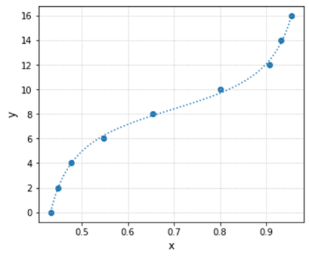
Running the program will generate a plot of the data points with the fitted curve, as well as some statistical information about the fit quality and the optimal coefficients.

Found solution in 43 function evaluations.
Both actual and predicted relative reductions
in the sum of squares are at most 0.000000

R-square = 0.9990, RMSE = 0.0065

Coefficients:
k  = 0.211
w  = 0.377
x0 = 8.565
y0 = 0.701


Tangent Function Fit

The same code can be used to fit a tangent function to a data set. All you need to do is replace the arctangent function with the tangent one and have the appropriate xdata and ydata. In this particular case, the previous data set arrays were just swapped. The program output after the modifications is also shown. The full code can be found on my GitHub repository.

# Defining parametrized tangent function
def f(x, k, w, x0, y0):
    return k * np.tan(w*(x-x0)) + y0

# Defining data points
xdata = [0.432, 0.448, 0.477, 0.547, 0.653, 0.800, 0.908, 0.933, 0.955]
ydata = [0, 2, 4, 6, 8, 10, 12, 14, 16]
Found solution in 54 function evaluations.
Both actual and predicted relative reductions
in the sum of squares are at most 0.000000

R-square = 0.9985, RMSE = 0.1998

Coefficients:
k  = 2.383
w  = 4.896
x0 = 0.696
y0 = 8.377


If we compare the coefficients from the arctangent fit with the ones from the tangent fit, using the relationships derived at the top of the post, they don’t quite match. Even when using the exact same data set by swapping xdata and ydata.

This result shouldn’t be a surprise, since the error between y values and their predictions, used inside the fitting algorithm, are not equivalent even with identical swapped data sets. Additionally, the distribution of the data points among the x coordinates also affects the optimal coefficient values of the fitted function.

Going from Arctangent to Tangent

Let’s take a closer look at the influence of the data point distribution on the resulting fitted function, and when we are better off using the coefficients of the function fitted to the inverse data set.

We want to fit a transfer function to the following data using the tangent function:

# Defining parametrized tangent function
def f(x, k, w, x0, y0):
    return k * np.tan(w*(x-x0)) + y0

# Defining data points
xdata = [0.700, 0.698, 0.691, 0.680, 0.654, 0.587, 0.504, 0.394, 0.341, 0.300, 0.282, 0.275, 0.272]
ydata = [0, 2, 4, 6, 8, 10, 12, 14, 16, 18, 20, 22, 24]

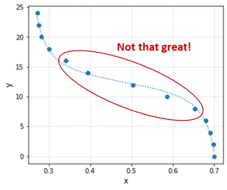
Using the Python program with the code snippet above substituted into it, we get the fit results below. Even though the R-square is a respectable value, the fitted function doesn’t do a good job capturing the transition between the two end states.

Found solution in 80 function evaluations.
Both actual and predicted relative reductions
in the sum of squares are at most 0.000000

R-square = 0.9959, RMSE = 0.4766

Coefficients:
k  = -2.143
w  = 6.469
x0 = 0.485
y0 = 12.382


Due to the overall shape of the transfer function and the fact that the data was originally collected at constant y increments, there is a high concentration of points along the x axis on both ends of the test data range. That leaves the region of interest (inside the red ellipse) with relatively fewer points, biasing the fitted function towards the low and high x value regions (outside the red ellipse).

One way to tackle this issue is by inverting the data set and using, in this case, the arctangent function:

# Defining parametrized arctangent function
def f(x, k, w, x0, y0):
    return k * np.arctan(w*(x-x0)) + y0

# Defining data points
xdata = [0, 2, 4, 6, 8, 10, 12, 14, 16, 18, 20, 22, 24]
ydata = [0.700, 0.698, 0.691, 0.680, 0.654, 0.587, 0.504, 0.394, 0.341, 0.300, 0.282, 0.275, 0.272]

The new fit is now done with x values that are evenly distributed, removing the bias that occurred when the tangent function was used.

Found solution in 60 function evaluations.
Both actual and predicted relative reductions
in the sum of squares are at most 0.000000

R-square = 0.9992, RMSE = 0.0049

Coefficients:
k  = -0.164
w  = 0.354
x0 = 12.253
y0 = 0.486


Finally, we can then use the coefficient relationships to go from arctangent, that produces a better overall data fit, to the desired tangent transfer function. The plot below shows the new tangent function in orange (using the arctangent coefficients) in contrast with the original one in blue.

Digital Filtering

Digital Filtering

After a continuous signal goes through an analog-to-digital conversion, additional digital filtering can be applied to improve the signal quality. Whether the signal is being used in a real-time application or has been collected for a later analysis, implementing a digital filter via software is quite straightforward. We already saw them being casually used in some of my previous posts, such as MCP3008 with Raspberry Pi. Now, let’s go over these types of filters in more detail. For the examples, we will be using the signal processing functions from the the SciPy Python package.

One of the drawbacks of digital filtering (or analog filtering, for that matter) is the introduction of a phase delay in the filtered signal.

The plots on the left illustrate what an actual filtered signal and its phase lag would look like (top), in contrast with an ideal filtered signal with no lag (bottom). While the ideal situation cannot be achieved with real-time signal processing, it can be achieved when processing signals that are already sampled and stored as a discrete sequence of numerical values.

Since the sequence from start to finish is available, the idea is to filter it once (causing a phase shift) and then filter the resulting sequence backwards (causing a phase shift again). Since the filtering is done both forward and backwards, the phase shifts cancel each other, thus resulting in a zero-phase filtered signal!

To see how it’s done, check out the filtfilt function and the very good application examples on the SciPy documentation. You can also go for the code used to generate the plots above on my GitHub page. I should note that I use filtfilt all the time in my signal processing endeavors. There’s a lot of information that can be extracted from a signal after you clean it up a little bit. If the time alignment between events is critical, avoiding a phase shift is the way to go.

Before we get into the real-time application of digital filters, let’s talk briefly about how they’re implemented. I’ll focus on filters that can be described as the difference equation below:

whereis the input sequence (raw signal) andis the output sequence (filtered signal). Before you abandon this webpage, let me rewrite the equation so we can start bringing it to a more applicable form. Since the idea is to find the outputas a function of its previous values and the input, we can go with:

It’s common to normalize the coefficients so . Also, for simplicity, consider a first order filter which, in terms of difference equations, only depends on the values of the current and last time steps, or and . Thus:

So, to build a first-order low-pass digital filter, all we need to do is determine the coefficients , and. Luckily for us, the SciPy MATLAB-Style filter design functions return those coefficients, reducing our task to just the implementation of the filter using Python. Before we go over a couple of code examples, let’s examine a first-order filter that I use quite a bit.

Backward Difference Digital Filter

Going from the continuous domain to the discrete domain involves a transformation where we approximate a continuous variable by its discrete equivalent. I will start with a first-order low-pass filter, by analyzing its continuous behavior, more specifically the response to a unit step input.

The continuous system response to the constant input is given by , whereis the response time of the filter and is related to the filter cutoff frequencyby:

The response time of the filter is the time it takes for the output to reach approximately 63 % of the final value. In the case of the graph above, the response time is 0.1 seconds. If you’re wondering where that comes from, just calculate the system response using .

The differential equation that corresponds to the first order continuous system in question is:

And here is where our discrete approximation ofusing backward difference (with sampling period) comes into play:

By also transformingandinto their discrete counterpartsand, we can arrive to the difference equation below, which represents the first-order low-pass digital filter, where we used backward difference to approximate. Remember that and are the discrete current and previous time steps.

Finally, solving forgives us an equation very similar to the one we saw at the end of the previous section. Note that the coefficients andare a function of the sampling rate and the filter response time (in this particular case).

What I like about this filter implementation is that it’s fairly straightforward to see that the outputis a weighed average of its previous valueand the current input value. Furthermore, the smaller the response time (), the faster the filter is (higher cutoff frequency) and the more it follows the input value. Conversely, the slower the filter (), the more the output takes into account the previous value.

The Python code below shows how to implement this filter by placing it inside an execution loop and running a step input excitation through it. It will produce the plot shown at the beginning of this section. I invite you to experiment with different response times (cutoff frequencies) and sampling periods.

import numpy as np
import matplotlib.pyplot as plt

# Creating time array for "continuous" signal
tstop = 1  # Signal duration (s)
Ts0 = 0.001  # "Continuous" time step (s)
Ts = 0.02  # Sampling period (s)
t = np.arange(0, tstop+Ts0, Ts0)

# First order continuous system response to unit step input
tau = 0.1  # Response time (s)
y = 1 - np.exp(-t/tau)  # y(t)

# Preallocating signal arrays for digital filter
tf = []
yf = []

# Initializing previous and current values
xcurr = 1  # x[n] (step input)
yfprev = 0  # y[n-1]
yfcurr = 0  # y[n]

# Executing DAQ loop
tprev = 0
tcurr = 0
while tcurr <= tstop:
    # Doing filter computations every `Ts` seconds
    if (np.floor(tcurr/Ts) - np.floor(tprev/Ts)) == 1:
        yfcurr = tau/(tau+Ts)*yfprev + Ts/(tau+Ts)*xcurr
        yfprev = yfcurr
    # Updating output arrays
    tf.append(tcurr)
    yf.append(yfcurr)
    # Updating previous and current "continuous" time steps
    tprev = tcurr
    tcurr += Ts0

# Creating Matplotlib figure
fig = plt.figure(
    figsize=(6.3, 2.8),
    facecolor='#f8f8f8',
    tight_layout=True)
# Adding and configuring axes
ax = fig.add_subplot(
    xlim=(0, max(t)),
    xlabel='Time (s)',
    ylabel='Output ( - )',
    )
ax.grid(linestyle=':')
# Plotting signals
ax.plot(t, y, linewidth=1.5, label='Continuous', color='#1f77b4')
ax.plot(tf, yf, linewidth=1.5, label='Discrete', color='#ff7f0e')
ax.legend(loc='lower right')

SciPy Butterworth Digital Filter

The non-functional code snippet below shows how to import the SciPy signal processing module an use it to create a first-order digital Butterworth filter. Note that the implementation of the filter in the DAQ execution loop is very similar to what was done in the example code above. In this particular case however, you should be able to immediately identify the difference equation for the filter

where the arrays containing the coefficients , and, are the output of the SciPy function signal.butter for the corresponding cutoff frequency and discrete sampling period.

# Importing SciPy module
from scipy import signal

#
# Doing other initialization
#

# Discrete signal parameters
tsample = 0.01  # Sampling period for code execution (s)
fs = 1/tsample  # Sampling frequency (Hz)

# Finding a, b coefficients for digital butterworth filter
fc = 10  # Low-pass cutoff frequency (Hz)
b, a = signal.butter(1, fc, fs=fs)

# Preallocating variables
xcurr = 0  # x[n]
ycurr = 0  # y[n]
xprev = 0  # x[n-1]
yprev = 0  # y[n-1]

tprev = 0
tcurr = 0
# Executing DAQ loop
while tcurr <= tstop:
    # Doing I/O tasks every `tsample` seconds
    if (np.floor(tcurr/tsample) - np.floor(tprev/tsample)) == 1:
        # Simulating DAQ device signal acquisition
        xcurr = mydaq.value
        # Filtering signal (digital butterworth filter)
        ycurr = -a[1]*yprev + b[0]*xcurr + b[1]*xprev
        yprev = ycurr
    # Updating previous values
    xprev = xcurr
    tprev = tcurr
    # Incrementing time step
    tcurr += Ts0

Finally, as I mentioned at the top, you can implement higher order or different types of filters. Take a look at the signal.iirnotch filter, which is a very useful design that removes specific frequencies from the original signal, such as the good old 60 Hz electric grid one.