
After a continuous signal goes through an analog-to-digital conversion, additional digital filtering can be applied to improve the signal quality. Whether the signal is being used in a real-time application or has been collected for a later analysis, implementing a digital filter via software is quite straightforward. We already saw them being casually used in some of my previous posts, such as MCP3008 with Raspberry Pi. Now, let’s go over these types of filters in more detail. For the examples, we will be using the signal processing functions from the the SciPy Python package.

One of the drawbacks of digital filtering (or analog filtering, for that matter) is the introduction of a phase delay in the filtered signal.
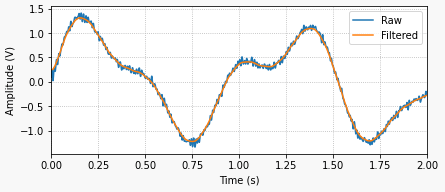
The plots on the left illustrate what an actual filtered signal and its phase lag would look like (top), in contrast with an ideal filtered signal with no lag (bottom). While the ideal situation cannot be achieved with real-time signal processing, it can be achieved when processing signals that are already sampled and stored as a discrete sequence of numerical values.
Since the sequence from start to finish is available, the idea is to filter it once (causing a phase shift) and then filter the resulting sequence backwards (causing a phase shift again). Since the filtering is done both forward and backwards, the phase shifts cancel each other, thus resulting in a zero-phase filtered signal!
To see how it’s done, check out the filtfilt function and the very good application examples on the SciPy documentation. You can also go for the code used to generate the plots above on my GitHub page. I should note that I use filtfilt all the time in my signal processing endeavors. There’s a lot of information that can be extracted from a signal after you clean it up a little bit. If the time alignment between events is critical, avoiding a phase shift is the way to go.
Before we get into the real-time application of digital filters, let’s talk briefly about how they’re implemented. I’ll focus on filters that can be described as the difference equation below:

where![]() is the input sequence (raw signal) and
is the input sequence (raw signal) and![]() is the output sequence (filtered signal). Before you abandon this webpage, let me rewrite the equation so we can start bringing it to a more applicable form. Since the idea is to find the output
is the output sequence (filtered signal). Before you abandon this webpage, let me rewrite the equation so we can start bringing it to a more applicable form. Since the idea is to find the output![]() as a function of its previous values and the input, we can go with:
as a function of its previous values and the input, we can go with:

It’s common to normalize the coefficients so ![]() . Also, for simplicity, consider a first order filter which, in terms of difference equations, only depends on the values of the current and last time steps, or
. Also, for simplicity, consider a first order filter which, in terms of difference equations, only depends on the values of the current and last time steps, or ![]() and
and ![]() . Thus:
. Thus:

So, to build a first-order low-pass digital filter, all we need to do is determine the coefficients ![]() ,
, ![]() and
and![]() . Luckily for us, the SciPy MATLAB-Style filter design functions return those coefficients, reducing our task to just the implementation of the filter using Python. Before we go over a couple of code examples, let’s examine a first-order filter that I use quite a bit.
. Luckily for us, the SciPy MATLAB-Style filter design functions return those coefficients, reducing our task to just the implementation of the filter using Python. Before we go over a couple of code examples, let’s examine a first-order filter that I use quite a bit.
Backward Difference Digital Filter
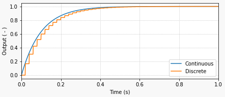
Going from the continuous domain to the discrete domain involves a transformation where we approximate a continuous variable by its discrete equivalent. I will start with a first-order low-pass filter, by analyzing its continuous behavior, more specifically the response to a unit step input.
The continuous system response to the constant input ![]() is given by
is given by ![]() , where
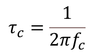
, where![]() is the response time of the filter and is related to the filter cutoff frequency
is the response time of the filter and is related to the filter cutoff frequency![]() by:
by:
The response time of the filter is the time it takes for the output to reach approximately 63 % of the final value. In the case of the graph above, the response time is 0.1 seconds. If you’re wondering where that comes from, just calculate the system response using ![]() .
.
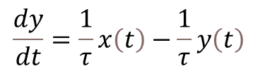
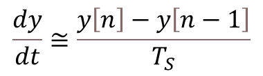
The differential equation that corresponds to the first order continuous system in question is:
And here is where our discrete approximation of![]() using backward difference (with sampling period
using backward difference (with sampling period![]() ) comes into play:
) comes into play:
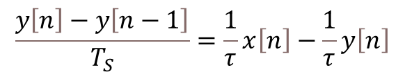
By also transforming![]() and
and![]() into their discrete counterparts
into their discrete counterparts![]() and
and![]() , we can arrive to the difference equation below, which represents the first-order low-pass digital filter, where we used backward difference to approximate
, we can arrive to the difference equation below, which represents the first-order low-pass digital filter, where we used backward difference to approximate![]() . Remember that
. Remember that ![]() and
and ![]() are the discrete current and previous time steps.
are the discrete current and previous time steps.
Finally, solving for![]() gives us an equation very similar to the one we saw at the end of the previous section. Note that the coefficients
gives us an equation very similar to the one we saw at the end of the previous section. Note that the coefficients ![]() and
and![]() are a function of the sampling rate and the filter response time (
are a function of the sampling rate and the filter response time (![]() in this particular case).
in this particular case).
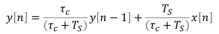
What I like about this filter implementation is that it’s fairly straightforward to see that the output![]() is a weighed average of its previous value
is a weighed average of its previous value![]() and the current input value
and the current input value![]() . Furthermore, the smaller the response time (
. Furthermore, the smaller the response time (![]() ), the faster the filter is (higher cutoff frequency) and the more it follows the input value. Conversely, the slower the filter (
), the faster the filter is (higher cutoff frequency) and the more it follows the input value. Conversely, the slower the filter (![]() ), the more the output takes into account the previous value.
), the more the output takes into account the previous value.
The Python code below shows how to implement this filter by placing it inside an execution loop and running a step input excitation through it. It will produce the plot shown at the beginning of this section. I invite you to experiment with different response times (cutoff frequencies) and sampling periods.
import numpy as np
import matplotlib.pyplot as plt

# Creating time array for "continuous" signal
tstop = 1  # Signal duration (s)
Ts0 = 0.001  # "Continuous" time step (s)
Ts = 0.02  # Sampling period (s)
t = np.arange(0, tstop+Ts0, Ts0)

# First order continuous system response to unit step input
tau = 0.1  # Response time (s)
y = 1 - np.exp(-t/tau)  # y(t)

# Preallocating signal arrays for digital filter
tf = []
yf = []

# Initializing previous and current values
xcurr = 1  # x[n] (step input)
yfprev = 0  # y[n-1]
yfcurr = 0  # y[n]

# Executing DAQ loop
tprev = 0
tcurr = 0
while tcurr <= tstop:
    # Doing filter computations every `Ts` seconds
    if (np.floor(tcurr/Ts) - np.floor(tprev/Ts)) == 1:
        yfcurr = tau/(tau+Ts)*yfprev + Ts/(tau+Ts)*xcurr
        yfprev = yfcurr
    # Updating output arrays
    tf.append(tcurr)
    yf.append(yfcurr)
    # Updating previous and current "continuous" time steps
    tprev = tcurr
    tcurr += Ts0

# Creating Matplotlib figure
fig = plt.figure(
    figsize=(6.3, 2.8),
    facecolor='#f8f8f8',
    tight_layout=True)
# Adding and configuring axes
ax = fig.add_subplot(
    xlim=(0, max(t)),
    xlabel='Time (s)',
    ylabel='Output ( - )',
    )
ax.grid(linestyle=':')
# Plotting signals
ax.plot(t, y, linewidth=1.5, label='Continuous', color='#1f77b4')
ax.plot(tf, yf, linewidth=1.5, label='Discrete', color='#ff7f0e')
ax.legend(loc='lower right')
SciPy Butterworth Digital Filter
The non-functional code snippet below shows how to import the SciPy signal processing module an use it to create a first-order digital Butterworth filter. Note that the implementation of the filter in the DAQ execution loop is very similar to what was done in the example code above. In this particular case however, you should be able to immediately identify the difference equation for the filter
where the arrays containing the coefficients ![]() ,
, ![]() and
and![]() , are the output of the SciPy function
, are the output of the SciPy function signal.butter for the corresponding cutoff frequency and discrete sampling period.
# Importing SciPy module
from scipy import signal

#
# Doing other initialization
#

# Discrete signal parameters
tsample = 0.01  # Sampling period for code execution (s)
fs = 1/tsample  # Sampling frequency (Hz)

# Finding a, b coefficients for digital butterworth filter
fc = 10  # Low-pass cutoff frequency (Hz)
b, a = signal.butter(1, fc, fs=fs)

# Preallocating variables
xcurr = 0  # x[n]
ycurr = 0  # y[n]
xprev = 0  # x[n-1]
yprev = 0  # y[n-1]

tprev = 0
tcurr = 0
# Executing DAQ loop
while tcurr <= tstop:
    # Doing I/O tasks every `tsample` seconds
    if (np.floor(tcurr/tsample) - np.floor(tprev/tsample)) == 1:
        # Simulating DAQ device signal acquisition
        xcurr = mydaq.value
        # Filtering signal (digital butterworth filter)
        ycurr = -a[1]*yprev + b[0]*xcurr + b[1]*xprev
        yprev = ycurr
    # Updating previous values
    xprev = xcurr
    tprev = tcurr
    # Incrementing time step
    tcurr += Ts0
Finally, as I mentioned at the top, you can implement higher order or different types of filters. Take a look at the signal.iirnotch filter, which is a very useful design that removes specific frequencies from the original signal, such as the good old 60 Hz electric grid one.

3 thoughts on “Digital Filtering”