In this simple hardware setup, we will explore different coding possibilities using a Raspberry Pi with only a push button and an LED. It will be a good opportunity to compare Python classes vs functions, with code that shows the benefits of the former. More specifically, classes offer modularity and the possibility of reuse through multiple instances.
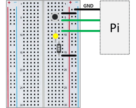
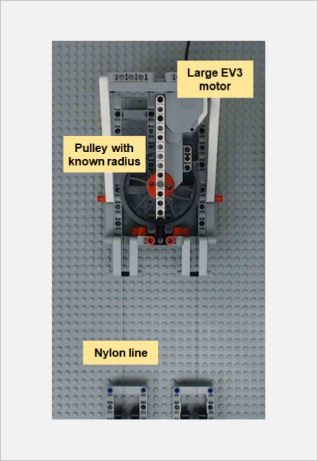
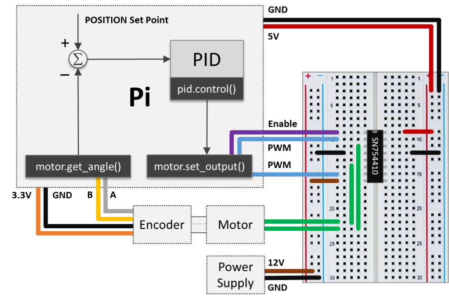
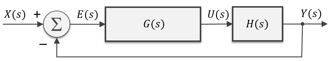
The diagram shows the very straightforward setup where the button and LED have one of their legs connected to a (distinct) GPIO pin and the other to a ground pin. A 330 Ω resistor must be connected in series with the LED, whose intensity is controlled by a PWM output. That is as simple as it gets.
Note: If the button doesn’t seem to be working, try connecting a different pair of legs, since some of them could be common.
While the dimmer functionality could be achieved using solely electronic circuitry and without a Raspberry Pi, the main point of this post is to explore coding and see what can be done with software!
Let’s start with the requirements of how we want the dimmer to work. By pressing and holding the button, the LED light intensity should increase linearly until reaching its maximum value and then decrease until it reaches its minimum value (LED off). This cycle repeats itself until the button is released, causing the light intensity to stay constant at its last value. By pressing the button again, the cycle resumes from where it stopped.
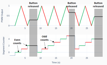
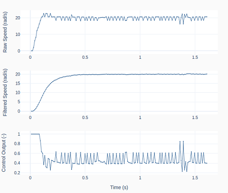
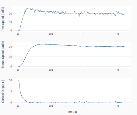
The plots provide a visual understanding of the requirements. The PWM output controlling the LED intensity ramps up (green) and down (red) while the button is pressed. As it is released, the last PWM output level is then held until the button is pressed again.
In terms of control logic, I use an integer to count ramp transitions. Even values correspond to upward ramps and odd values to downward ramps. Every time the button is released and then pressed again, the counter is reset to zero.
There are two main components in the control logic for the dimmer:
- The
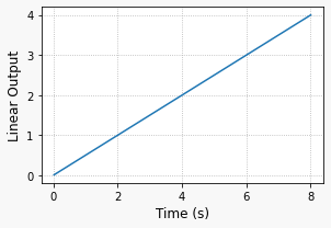
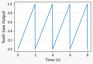
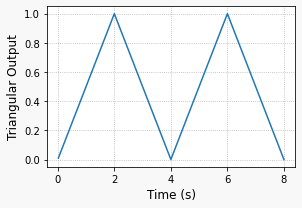
calc_ramp()function that creates the triangular wave output in three steps. 1) Linear output generation, 2) Converting linear output to a tooth saw wave, thus limiting it between 0 and 1, and 3) Flipping odd count sections to generate a triangular wave.
- Time shifting and counter reset to ensure smooth transitions every time the button is released and then pressed again. When a ramp is interrupted due to a button release event, it it will restart from where it stopped so the effective ramp duration (discounting the elapsed released time) is always the same.
Python Function
The code below shows how the function calc_ramp() and the time shifting are integrated inside an execution loop that controls the LED light intensity. As usual, the interface with the Raspberry Pi is done using GPIO Zero classes, more specifically DigitalInputDevice for the button pin and PWMOutputDevice for the LED pin.
# Importing modules and classes
import time
import numpy as np
from gpiozero import DigitalInputDevice, PWMOutputDevice
from utils import plot_line
# Assigning dimmer parameter values
pinled = 17 # PWM output (LED input) pin
pinbutton = 5 # button input pin
pwmfreq = 200 # PWM frequency (Hz)
pressedbefore = False # Previous button pressed state
valueprev = 0 # Previous PWM value
kprev = 0 # Previous PWM ramp segmment counter
tshift = 0 # PWM ramp time shift (to start where it left off)
tramp = 2 # PWM output 0 to 100% ramp time (s)
# Assigning execution loop parameter values
tsample = 0.02 # Sampling period for code execution (s)
tstop = 30 # Total execution time (s)
# Preallocating output arrays for plotting
t = [] # Time (s)
value = [] # PWM output duty cycle value
k = [] # Ramp segment counter
def calc_ramp(t, tramp):
"""
Creates triangular wave output with amplitude 0 to 1 and period 2 x tramp.
"""
# Creating linear output so the value is 1 when t=tramp
valuelin = t/tramp
# Creating time segment counter
k = t//tramp
# Shifting output down by number of segment counts
value = valuelin - k
# Flipping odd count output to create triangular wave
if (k % 2) == 1:
value = 1 - value
return value, k
# Creating button and PWM output (LED input) objects
button = DigitalInputDevice(pinbutton, pull_up=True, bounce_time=0.1)
led = PWMOutputDevice(pinled, frequency=pwmfreq)
# Initializing timers and starting main clock
tpressed = 0
tprev = 0
tcurr = 0
tstart = time.perf_counter()
# Initializing PWM value and ramp time segment counter
valuecurr = 0
kcurr = -1
# Executing loop
print('Running code for', tstop, 'seconds ...')
while tcurr <= tstop:
# Executing code every `tsample` seconds
if (np.floor(tcurr/tsample) - np.floor(tprev/tsample)) == 1:
# Getting button properties only once
pressed = button.is_active
# Checking for button press
if pressed and not pressedbefore:
# Calculating ramp time shift based on last PWM value
if (kprev % 2) == 0:
tshift = valueprev*tramp
else:
tshift = (1-valueprev)*tramp + tramp
# Starting pressed button timer
tpressed = time.perf_counter() - tstart
# Updating previous button state
pressedbefore = True
# Checking for button release
if not pressed and pressedbefore:
# Storing PWM value and ramp segment counter
valueprev = led.value
kprev = kcurr
# Updating previous button state
pressedbefore = False
# Updating PWM output (LED intensity)
if pressed:
valuecurr, kcurr = calc_ramp(tcurr-tpressed+tshift, tramp)
led.value = valuecurr
# Appending current values to output arrays
t.append(tcurr)
value.append(valuecurr)
k.append(kcurr)
# Updating previous time and getting new current time (s)
tprev = tcurr
tcurr = time.perf_counter() - tstart
print('Done.')
# Releasing pins
led.close()
button.close()
# Plotting results
plot_line([t]*2, [value, k],
yname=['PWM Output', 'Segment Counter'], axes='multi')
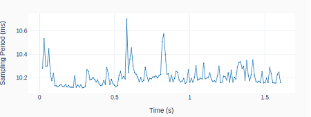
plot_line([t[1::]], [1000*np.diff(t)], yname=['Sampling Period (ms)'])
Python Class
Having the function and the time shifting “mixed” with the code makes for a less clean execution loop section, which can get pretty busy if there are more devices being controlled inside of it. The next piece of code shows how to integrate the two main components of the dimmer control inside a Python class. In addition to removing complexity from the execution loop, it makes it really easy to run multiple dimmers at the same time! This circles back to the modularity that was mentioned at the top of the post. You can create different classes for more complex devices and have them all be part of a module, such as gpiozero_extended.py. In the example below, I create two LED dimmer objects that can be controlled independently.
# Importing modules and classes
import time
import numpy as np
from gpiozero import DigitalInputDevice, PWMOutputDevice


class Dimmer:
    """
    Class that represents an LED dimmer.

    """
    def __init__(self, pinbutton=None, pinled=None):
        # Assigning GPIO pins
        self._pinbutton = pinbutton  # button input pin
        self._pinled = pinled  # PWM output (LED input) pin
        # Assigning dimmer parameter values
        self._pwmfreq = 200  # PWM frequency (Hz)
        self._tshift = 0  # PWM ramp time shift (to start where it left off)
        self._tramp = 2  # PWM output 0 to 100% ramp time (s)
        self._tpressed = 0  # Time button was pressed (s)
        self._tstart = 0  # Starting time of dimmer execution
        self._pressed = False  # Current button pressed state
        self._pressedbefore = False  # Previous button pressed state
        self._valueprev = 0  # Previous PWM value
        self._kcurr = -1  # Current PWM ramp segment counter
        self._kprev = 0  # Previous PWM ramp segmment counter
        # Creating button and PWM output (LED input) objects
        self._button = DigitalInputDevice(self._pinbutton, pull_up=True, bounce_time=0.1)
        self._led = PWMOutputDevice(self._pinled, frequency=self._pwmfreq)

    def _calc_ramp_value(self, t):
        # Creating linear output so the value is 1 when t=tramp
        valuelin = t/self._tramp
        # Creating time segment counter
        self._kcurr = t//self._tramp
        # Shifting output down by number of segment counts
        value = valuelin - self._kcurr
        # Flipping odd count output to create triangular wave
        if (self._kcurr % 2) == 1:
            value = 1 - value
        return value

    def reset_timer(self, tstart):
        # Resets dimmer timer to `tstart`
        self._tstart = tstart

    def update_value(self, t):
        # Getting button properties only once
        self._pressed = self._button.is_active
        # Checking for button press
        if self._pressed and not self._pressedbefore:
            # Calculating ramp time shift based on last PWM value
            if (self._kprev % 2) == 0:
                self._tshift = self._valueprev*self._tramp
            else:
                self._tshift = (1-self._valueprev)*self._tramp + self._tramp
            # Starting pressed button timer
            self._tpressed = time.perf_counter() - self._tstart
            # Updating previous button state
            self._pressedbefore = True
        # Checking for button release
        if not self._pressed and self._pressedbefore:
            # Storing PWM value and ramp segment counter
            self._valueprev = self._led.value
            self._kprev = self._kcurr
            # Updating previous button state
            self._pressedbefore = False
        # Updating PWM output (LED intensity)
        if self._pressed:
            self._led.value = self._calc_ramp_value(t-self._tpressed+self._tshift)

    def __del__(self):
        self._button.close()
        self._led.close()


# Assigning execution loop parameter values
tsample = 0.02 # Sampling period for code execution (s)
tstop = 30 # Total execution time (s)

# Creating dimmer objects
dimmer1 = Dimmer(pinled=17, pinbutton=5)
dimmer2 = Dimmer(pinled=18, pinbutton=6)

# Initializing timers and starting main clock
tprev = 0
tcurr = 0
tstart = time.perf_counter()
# Resettting dimmer timer
dimmer1.reset_timer(tstart)
dimmer2.reset_timer(tstart)

# Executing loop
print('Running code for', tstop, 'seconds ...')
while tcurr <= tstop:
    # Executing code every `tsample` seconds
    if (np.floor(tcurr/tsample) - np.floor(tprev/tsample)) == 1:
        # Updating dimmer outputs
        dimmer1.update_value(tcurr)
        dimmer2.update_value(tcurr)
    # Updating previous time and getting new current time (s)
    tprev = tcurr
    tcurr = time.perf_counter() - tstart
print('Done.')

# Releasing pins
del dimmer1
del dimmer2
If you watch the video, you’ll notice that the light intensity change is not as linear as one would expect, even when the PWM output is. One way to improve this is to add a non-linear transfer function between the ramp function output and the actual PWM set point value.
Also, it would be nice to have the ability to switch the dimmer off by, for instance, pressing and releasing the button for a short period of time. The improved class that does that can be found on my GitHub page.