
In this first of two posts, we’ll go over the simplifications of the equations that govern the dynamic behavior of a DC motor. By doing so, we should be able to use a non-intrusive and fairly straightforward approach to determine the parameters that characterize the motor from a control systems stand point.
While this might get a bit arid at times, I’ll try to keep it interesting by using some real motor parameters and Simulink to show the impact of the simplifications as we move towards our final dynamic system equation. Let’s start with the well known coupled differential equations (which are essentially a mathematical representation) for the electric motor:

Where (in SI units, for good measure):

By applying the Laplace transformation to the equations above and rearranging them in a way that they are solved for the angular velocity and current, we get:

and therefore

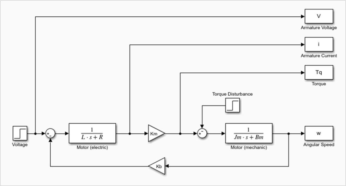
The rearranged equations can then be represented in the form of a block diagram, which will come in handy when we talk about the model simplification. Also, note the negative “feedback” nature of the back EMF term![]() (which makes the rotor speed inherently stable to small disturbances in the load torque).
(which makes the rotor speed inherently stable to small disturbances in the load torque).

The DC motor has two time constants associated with its dynamic behavior. The electrical time constant![]() (directly obtained from one of the first-order blocks in the diagram) and the mechanical time constant
(directly obtained from one of the first-order blocks in the diagram) and the mechanical time constant![]() , which is not so intuitive and we’ll see later where it comes from.
, which is not so intuitive and we’ll see later where it comes from.
Especially for smaller motors, the electrical time constant is substantially faster than the mechanical time constant. That is generally accompanied by![]() , which means that the corresponding inductance term in the first-order block can be neglected. The block diagram of the resulting system is shown next.
, which means that the corresponding inductance term in the first-order block can be neglected. The block diagram of the resulting system is shown next.

It’s time to put some numbers into these two models and observe how they behave when simulated using Simulink. In order to do that, I found myself a motor data sheet for permanent magnet DC motors from Moog. These tend to be very high end components when compared to the DC motors I’ve been using in my previous posts. I.e. they are designed for a more professional application. Not for the “DIY-finite-budget-hobbyist”, like myself!
With that said, I chose the smallest and the largest motors from the catalog, whose parameters are summarized below:
| C23-L33-W10 | C42-L90-W30 | ||
| Length | mm | 85 | 229 |
| Diameter | mm | 57 | 102 |
| Armature Voltage | V (DC) | 12 | 90 |
| Rated Current | A | 4.75 | 5 |
| Rated Speed | rad/s | 492 | 159 |
| Rated Torque | N.m | 0.05 | 2.26 |
| Friction Torque | N.m | 0.02 | 0.17 |
| Torque Constant ( | N.m/A | 0.0187 | 0.5791 |
| Back EMF Constant ( | V/rad/s | 0.0191 | 0.5730 |
| Armature Resistance ( | Ohm | 0.60 | 1.45 |
| Armature Inductance ( | H | 0.35e-3 | 5.4e-3 |
| Rotor Inertia ( | kg.m2 | 1.554e-5 | 2.189e-3 |
| Damping Coefficient ( | N.m/rad/s | 1e-5 | 6.8e-4 |
| Electrical Time Constant ( | ms | 0.58 | 3.72 |
| Mech. Time Constant ( | ms | 25.7 | 9.54 |
Taking a closer look at the last two rows, the electrical time constant of the smaller motor is significantly faster than its mechanical time constant, especially when compared to the larger motor. We will see how that plays out in a bit.
Also, for the simulation, the two inputs are the armature voltage and the load (or disturbance) torque, the latter accounting for the friction torque as well. The outputs are shown in the Simulink model picture below. The armature current and angular speed are the ones of most interest for checking the validity of the model against the data sheet values. In other words, when running the model with only voltage and torque as inputs, everything else should “fall in place”, matching the table data.
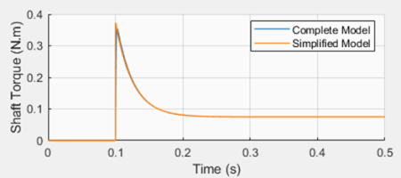
Small DC Motor Simulation Results
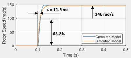
The plots show the simulation results for a step response with the armature voltage (12 V) and rated torque (0.05 N.m) for the small C23-L33-W10 motor. Two Simulink models were used: the complete model (shown above) and the simplified one (not shown here). Both can be found on my GitHub page.
The first takeaway is that the final rotor speed and armature current agree well with the corresponding rated values in the table. Also, the response time of 25.6 ms correlates fairly well with what is, in this particular case, the mechanical response time in the table.

While the simulated steady-state rotor speed is very close to the table value (502 vs 492 rpm), the armature current correlation is not so stellar (4.0 vs. 4.75 A) yet still satisfactory. It should be noted that the table values are probably obtained from actual motor tests or from a more sophisticated model.
The second takeaway is that the reduced order model produces virtually the same results as the complete model.

Large DC Motor Simulation Results
The large motor C42-L90-W30 simulation results show that, when the electrical and mechanical time constants are comparable, the simplified model cannot capture the dynamic behavior of the motor, as it was the case with the small motor.
However, the steady-state values still correlate fairly well with the published table values. A rotor speed of 146 rad/s vs. 159 rad/s, and an armature current of 4.37 A vs. 5 A.
As alluded to in the previous case, even the complete model used in the simulation is still an approximation when it comes to accurately describing the behavior of the DC motor.


Simplified DC Motor Model
With the simulation results in mind, we can use the simplified (or reduced order) model to describe the dynamic response of the types of DC motors that I’ll be dealing with throughout my blog.
From the block diagram it’s possible to write:

And rearranging:

Doing the inverse Laplace Transform to put in back in differential equation form:

or

Where:

As a quick note, if we take a closer look at the reduced model, we can identify the mechanical time constant![]() , in the particular case where there are no additional rotating inertias reduced to the rotor shaft.
, in the particular case where there are no additional rotating inertias reduced to the rotor shaft.
At this point, the motor can be characterized if we determine the values for![]() ,
,![]() and
and![]() . There are three non-intrusive tests that can be done with an actual motor, from which the three aforementioned parameters can be extracted.
. There are three non-intrusive tests that can be done with an actual motor, from which the three aforementioned parameters can be extracted.
The first test is a torque stall test (![]() ) which reduces our last differential equation to:
) which reduces our last differential equation to:

From which![]() can be determined for a given input voltage and the corresponding load torque that causes the DC motor to stall.
can be determined for a given input voltage and the corresponding load torque that causes the DC motor to stall.
The second test is a steady-state test (![]() ) with no load torque, which gives us:
) with no load torque, which gives us:

Since![]() is known from the previous test and the angular velocity can be measured for a given input voltage, the parameter
is known from the previous test and the angular velocity can be measured for a given input voltage, the parameter![]() can therefore be determined.
can therefore be determined.
The third test is a transient step-input test with no load, which reduces our simplified equation to:

By measuring the response time ![]() of the first-order system,
of the first-order system,![]() can be finally determined (since
can be finally determined (since![]() is already known at this point).
is already known at this point).
Final Remarks
We have seen how it’s possible to determine, or better said estimate, the main parameters ![]() ,
, ![]() and
and![]() for the reduced order model of a DC motor. This can be accomplished without having to disassemble the motor to measure the rotor moment of inertia, or having a more sophisticated electrical measurement setup to determine the armature inductance.
for the reduced order model of a DC motor. This can be accomplished without having to disassemble the motor to measure the rotor moment of inertia, or having a more sophisticated electrical measurement setup to determine the armature inductance.

The three tests described above can be performed on a simple test bench. Part 2 of this post will go over an experimental setup with the LEGO EV3 large motor and some automated testing using the pyev3 python package. Stay tuned!
