Tag: Raspberry Pi

Pulse Rate Monitor with Raspberry Pi

Pulse Rate Monitor with Raspberry Pi

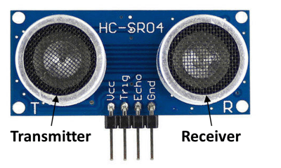
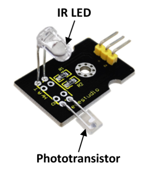
Pulse rate can be detected using a variety of physical principles. One way of doing it is by applying infrared light to one side of the tip of your finger and sensing the “output” on the other side with a phototransistor. The blood flow through the capillaries at the finger tip fluctuates with the same frequency (rate) of your pulse. That fluctuation can be detected after processing the signal captured by the sensor.

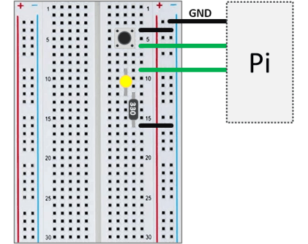
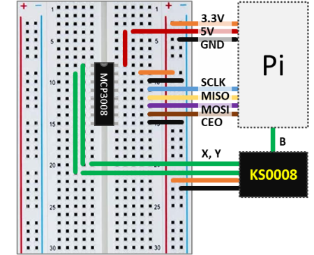
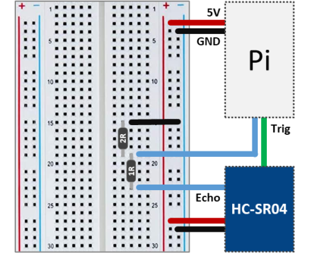
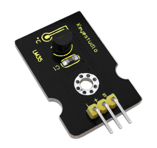
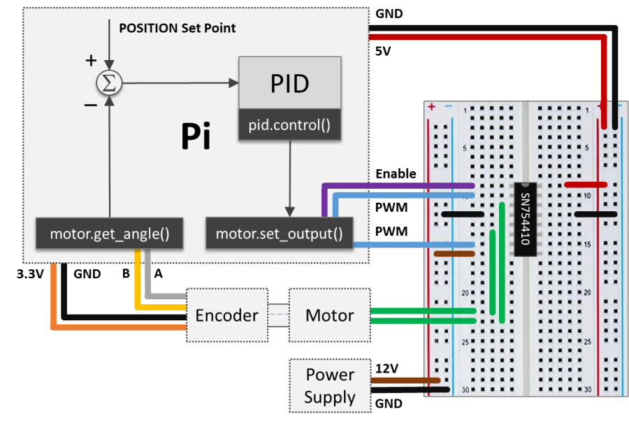
Keyestudio has a rudimentary pulse rate monitor (KS0015) that does the trick. In this post we will go over the signal processing and how to display the pulse rate in real time. Since the KS0015 outputs an analog signal, it has to be used with the MCP3008 analog-to-digital converter chip, as illustrated in the schematics below.

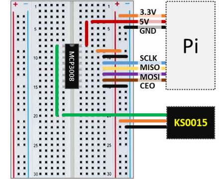
As noted in previous posts, adopting a reference voltage of 3.3V for the MCP3008 provides the best resolution for the analog-to-digital conversion. The sensor output therefore has to be no greater than 3.3V, which can be achieved by using 3.3 instead of 5V as the supply voltage for the KS0015.

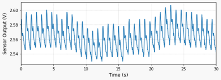
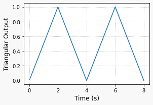
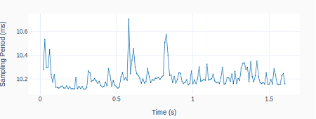
The very first thing to do is to look at the signal coming from the sensor as the tip of my index finger is placed between the IR LED and the phototransistor. The plot on the left can be generated by running the Python code below.

By inspecting the program, the first thing to observe is the sampling period (tsample) of 0.02 s. Since we don’t know much about the signal, it’s always good to start with a smaller value. The second thing is the wait time of 5 seconds before collecting any data. After tinkering around for a bit, I realized that the sensor is very sensitive to finger movements. Therefore, waiting for the signal to “settle down” really helps.

# Importing modules and classes
import time
import numpy as np
import matplotlib.pyplot as plt
from gpiozero import MCP3008


# Defining function for plotting
def make_fig():
    # Creating Matplotlib figure
    fig = plt.figure(
        figsize=(8, 3),
        facecolor='#f8f8f8',
        tight_layout=True)
    # Adding and configuring axes
    ax = fig.add_subplot(xlim=(0, max(t)))
    ax.set_xlabel('Time (s)', fontsize=12)
    ax.grid(linestyle=':')
    # Returning axes handle
    return ax


# Creating object for the pulse rate sensor output
vch = MCP3008(channel=0, clock_pin=11, mosi_pin=10, miso_pin=9, select_pin=8)

# Assigning some parameters
tsample = 0.02  # Sampling period for code execution (s)
tstop = 30  # Total execution time (s)
vref = 3.3  # Reference voltage for MCP3008
# Preallocating output arrays for plotting
t = []  # Time (s)
v = []  # Sensor output voltage (V)

# Waiting for 5 seconds for signal stabilization
time.sleep(5)

# Initializing variables and starting main clock
tprev = 0
tcurr = 0
tstart = time.perf_counter()
# Running execution loop
print('Running code for', tstop, 'seconds ...')
while tcurr <= tstop:
    # Getting current time (s)
    tcurr = time.perf_counter() - tstart
    # Doing I/O and computations every `tsample` seconds
    if (np.floor(tcurr/tsample) - np.floor(tprev/tsample)) == 1:
        # Getting current sensor voltage
        valuecurr = vref * vch.value
        # Assigning current values to output arrays
        t.append(tcurr)
        v.append(valuecurr)
    # Updating previous time value
    tprev = tcurr

print('Done.')
# Releasing GPIO pins
vch.close()

# Plotting results
ax = make_fig()
ax.set_ylabel('Sensor Output (V)', fontsize=12)
ax.plot(t, v, linewidth=1.5, color='#1f77b4')
ax = make_fig()
ax.set_ylabel('Sampling Period (ms)', fontsize=12)
ax.plot(t[1::], 1000*np.diff(t), linewidth=1.5, color='#1f77b4')

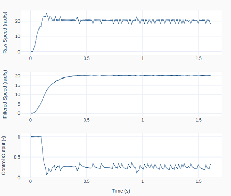
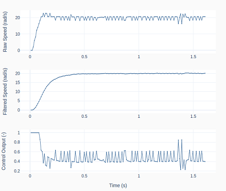
Digital Filtering and Pulse Detection

In this stage of the signal processing, let’s put some of the content of previous posts to good use. More specifically digital band-pass filtering and event detection for the pulse signal.

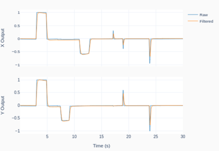
First let’s remove the low and high frequency components of the signal that are outside the band of interest. I chose 0.5 and 5 Hz (30 and 300 beats per minute) as the cutoff frequencies. That seems to be a reasonable bandwidth to account for the filter attenuation at the cutoff frequencies, as well as for the human heart “range of operation”.

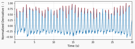
Then, let’s calculate the derivative of the signal so it’s easier to detect the pulse events. By normalizing the derivative based on its maximum value, the signal amplitude becomes more consistent and therefore a single value threshold can be used. In this case 25% of the maximum value.

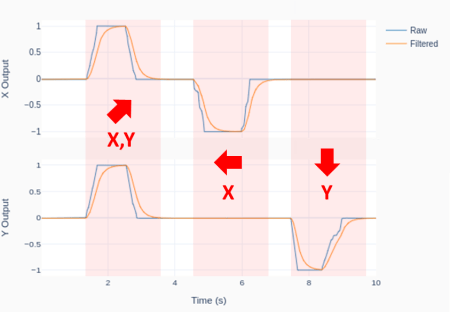
The plot on the top shows the normalized derivative of the filtered signal. In red are the trigger events detected by the function find_cluster, which I placed inside the module utils.py . As usual, all the code for this post can be found on my GitHub page.

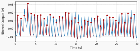
The plot on the bottom shows the identified trigger events (red dots) displayed on the filtered sensor output signal.

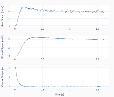
The Python program below is an extension of the one in the previous section, where the digital filter and the trigger detection features are now incorporated. The pulse rate is calculated using the median of the time difference between two consecutive trigger events. In this case, using the median instead of the mean is recommended since it makes the calculation more robust to outliers.

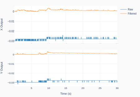
Running the code will generate the two graphs shown above and print the median pulse rate for the corresponding (30-second) data acquisition window. You will notice that the signal amplitude is fairly small (approx. 30 mV) and very sensitive to the finger tip location. It might take a few tries to find the correct position and pressure for the finger.

# Importing modules and classes
import time
import numpy as np
import matplotlib.pyplot as plt
from gpiozero import MCP3008
from utils import find_cluster


# Defining function for plotting
def make_fig():
    # Creating Matplotlib figure
    fig = plt.figure(
        figsize=(8, 3),
        facecolor='#f8f8f8',
        tight_layout=True)
    # Adding and configuring axes
    ax = fig.add_subplot(xlim=(0, max(t)))
    ax.set_xlabel('Time (s)', fontsize=12)
    ax.grid(linestyle=':')
    # Returning axes handle
    return ax


# Creating object for the pulse rate sensor output
vch = MCP3008(channel=0, clock_pin=11, mosi_pin=10, miso_pin=9, select_pin=8)

# Assigning some parameters
tsample = 0.1  # Sampling period for code execution (s)
tstop = 30  # Total execution time (s)
vref = 3.3  # Reference voltage for MCP3008
# Preallocating output arrays for plotting
t = np.array([])  # Time (s)
v = np.array([])  # Sensor output voltage (V)
vfilt = np.array([])  # Filtered sensor output voltage (V)

# Waiting for 5 seconds for signal stabilization
time.sleep(5)

# First order digital band-pass filter parameters
fc = np.array([0.5, 5])  # Filter cutoff frequencies (Hz)
tau = 1/(2*np.pi*fc)  # Filter time constants (s)
# Filter difference equation coefficients
a0 = tau[0]*tau[1]+(tau[0]+tau[1])*tsample+tsample**2
a1 = -(2*tau[0]*tau[1]+(tau[0]+tau[1])*tsample)
a2 = tau[0]*tau[1]
b0 = tau[0]*tsample
b1 = -tau[0]*tsample
# Assigning normalized coefficients
a = np.array([1, a1/a0, a2/a0])
b = np.array([b0/a0, b1/a0])
# Initializing filter values
x = [vref*vch.value] * len(b)  # x[n], x[n-1]
y = [0] * len(a)  # y[n], y[n-1], y[n-2]
time.sleep(tsample)

# Initializing variables and starting main clock
tprev = 0
tcurr = 0
tstart = time.perf_counter()
# Running execution loop
print('Running code for', tstop, 'seconds ...')
while tcurr <= tstop:
    # Getting current time (s)
    tcurr = time.perf_counter() - tstart
    # Doing I/O and computations every `tsample` seconds
    if (np.floor(tcurr/tsample) - np.floor(tprev/tsample)) == 1:
        # Getting current sensor voltage
        valuecurr = vref * vch.value
        # Assigning sensor voltage output to input signal array
        x[0] = valuecurr
        # Filtering signals
        y[0] = -np.sum(a[1::]*y[1::]) + np.sum(b*x)
        # Updating output arrays
        t = np.concatenate((t, [tcurr]))
        v = np.concatenate((v, [x[0]]))
        vfilt = np.concatenate((vfilt, [y[0]]))
        # Updating previous filter output values
        for i in range(len(a)-1, 0, -1):
            y[i] = y[i-1]
        # Updating previous filter input values
        for i in range(len(b)-1, 0, -1):
            x[i] = x[i-1]
    # Updating previous time value
    tprev = tcurr

print('Done.')
# Releasing pins
vch.close()

# Calculating and normalizing sensor signal derivative
dvdt = np.gradient(vfilt, t)
dvdt = dvdt/np.max(dvdt)
# Finding heart rate trigger event times
icl, ncl = find_cluster(dvdt>0.25, 1)
ttrigger = t[icl]
# Calculating heart rate (bpm)
bpm = 60/np.median(np.diff(ttrigger))
print("Heart rate = {:0.0f} bpm".format(bpm))

# Plotting results
ax = make_fig()
ax.set_ylabel('Normalized Derivative ( - )', fontsize=12)
ax.plot(t, dvdt, linewidth=1.5, color='#1f77b4', zorder=0)
for ik, nk in zip(icl, ncl):
    if ik+nk < len(t):
        ax.plot(t[ik:ik+nk], dvdt[ik:ik+nk], color='#aa0000')
ax = make_fig()
ax.set_ylabel('Filtered Output (V)', fontsize=12)
ax.plot(t, vfilt, linewidth=1.5, color='#1f77b4', zorder=0)
for ik, nk in zip(icl, ncl):
    ax.plot(t[ik:ik+nk], vfilt[ik:ik+nk], color='#aa0000')
    ax.scatter(t[ik+1], vfilt[ik+1], s=25, c='#aa0000')

Real-time Pulse Rate Detection

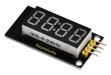
Now that we have the pulse rate detection and calculation working, we can modify the code from the previous section to add the real-time display of the pulse rate. For this step, we will use a 7-segment LED display with a TM1637 chip. In case you don’t have one, all the calls for the tm object in the code below should be removed and a simple

print("Heart rate = {:0.0f} bpm".format(bpm))

can be used to replace the code line

tm.number(int(bpm))

Also, notice how we are using a circular buffer (tbuffer) of 20 seconds that holds the signal for the pulse rate calculation. The buffer is updated every tsample seconds and the actual pulse rate calculation occurs every tdisp seconds. Through comparison with the previous program, you can see how the bpm calculation is now placed inside the execution loop, hence happening in real-time.

# Importing modules and classes
import time
import numpy as np
import matplotlib.pyplot as plt
import tm1637
from gpiozero import MCP3008
from utils import find_cluster


# Defining function for plotting
def make_fig():
    # Creating Matplotlib figure
    fig = plt.figure(
        figsize=(8, 3),
        facecolor='#f8f8f8',
        tight_layout=True)
    # Adding and configuring axes
    ax = fig.add_subplot(xlim=(0, max(t)))
    ax.set_xlabel('Time (s)', fontsize=12)
    ax.grid(linestyle=':')
    # Returning axes handle
    return ax


# Creating object for the pulse rate sensor output and LED display
vch = MCP3008(channel=0, clock_pin=11, mosi_pin=10, miso_pin=9, select_pin=8)
tm = tm1637.TM1637(clk=18, dio=17)

# Assigning some parameters
tsample = 0.1  # Sampling period for code execution (s)
tstop = 60  # Total execution time (s)
tbuffer = 20  # Data buffer length(s)
tdisp = 1  # Display update period (s)
vref = 3.3  # Reference voltage for MCP3008
# Preallocating circular buffer arrays for real-time processing
t = np.array([])  # Time (s)
v = np.array([])  # Sensor output voltage (V)
vfilt = np.array([])  # Filtered sensor output voltage (V)

# Waiting for 5 seconds for signal stabilization
time.sleep(5)

# First order digital band-pass filter parameters
fc = np.array([0.5, 5])  # Filter cutoff frequencies (Hz)
tau = 1/(2*np.pi*fc)  # Filter time constants (s)
# Filter difference equation coefficients
a0 = tau[0]*tau[1]+(tau[0]+tau[1])*tsample+tsample**2
a1 = -(2*tau[0]*tau[1]+(tau[0]+tau[1])*tsample)
a2 = tau[0]*tau[1]
b0 = tau[0]*tsample
b1 = -tau[0]*tsample
# Assigning normalized coefficients
a = np.array([1, a1/a0, a2/a0])
b = np.array([b0/a0, b1/a0])
# Initializing filter values
x = [vref*vch.value] * len(b)  # x[n], x[n-1]
y = [0] * len(a)  # y[n], y[n-1], y[n-2]
time.sleep(tsample)

# Initializing variables and starting main clock
tprev = 0
tcurr = 0
tstart = time.perf_counter()
# Running execution loop
tm.show('Hold')
print('Running code for', tstop, 'seconds ...')
print('Waiting', tbuffer, 'seconds for buffer fill.')
while tcurr <= tstop:
    # Getting current time (s)
    tcurr = time.perf_counter() - tstart
    # Doing I/O and computations every `tsample` seconds
    if (np.floor(tcurr/tsample) - np.floor(tprev/tsample)) == 1:
        # Getting current sensor voltage
        valuecurr = vref * vch.value
        # Assigning sensor voltage output to input signal array
        x[0] = valuecurr
        # Filtering signals
        y[0] = -np.sum(a[1::]*y[1::]) + np.sum(b*x)
        # Updating circular buffer arrays
        if len(t) == tbuffer/tsample:
            t = t[1::]
            v = v[1::]
            vfilt = vfilt[1::]
        t = np.concatenate((t, [tcurr]))
        v = np.concatenate((v, [x[0]]))
        vfilt = np.concatenate((vfilt, [y[0]]))
        # Updating previous filter output values
        for i in range(len(a)-1, 0, -1):
            y[i] = y[i-1]
        # Updating previous filter input values
        for i in range(len(b)-1, 0, -1):
            x[i] = x[i-1]
    # Processing signal in the buffer every `tdisp` seconds
    if ((np.floor(tcurr/tdisp) - np.floor(tprev/tdisp)) == 1) & (tcurr > tbuffer):
        # Calculating and normalizing sensor signal derivative
        dvdt = np.gradient(vfilt, t)
        dvdt = dvdt/np.max(dvdt)
        # Finding heart rate trigger event times
        icl, ncl = find_cluster(dvdt>0.25, 1)
        ttrigger = t[icl]
        # Calculating and displaying pulse rate (bpm)
        bpm = 60/np.median(np.diff(ttrigger))
        tm.number(int(bpm))
    # Updating previous time value
    tprev = tcurr

print('Done.')
tm.show('Done')
# Releasing pins
vch.close()
LED Dimmer with Raspberry Pi

LED Dimmer with Raspberry Pi

In this simple hardware setup, we will explore different coding possibilities using a Raspberry Pi with only a push button and an LED. It will be a good opportunity to compare Python classes vs functions, with code that shows the benefits of the former. More specifically, classes offer modularity and the possibility of reuse through multiple instances.

The diagram shows the very straightforward setup where the button and LED have one of their legs connected to a (distinct) GPIO pin and the other to a ground pin. A 330 Ω resistor must be connected in series with the LED, whose intensity is controlled by a PWM output. That is as simple as it gets.

Note: If the button doesn’t seem to be working, try connecting a different pair of legs, since some of them could be common.

While the dimmer functionality could be achieved using solely electronic circuitry and without a Raspberry Pi, the main point of this post is to explore coding and see what can be done with software!

Let’s start with the requirements of how we want the dimmer to work. By pressing and holding the button, the LED light intensity should increase linearly until reaching its maximum value and then decrease until it reaches its minimum value (LED off). This cycle repeats itself until the button is released, causing the light intensity to stay constant at its last value. By pressing the button again, the cycle resumes from where it stopped.

The plots provide a visual understanding of the requirements. The PWM output controlling the LED intensity ramps up (green) and down (red) while the button is pressed. As it is released, the last PWM output level is then held until the button is pressed again.

In terms of control logic, I use an integer to count ramp transitions. Even values correspond to upward ramps and odd values to downward ramps. Every time the button is released and then pressed again, the counter is reset to zero.

There are two main components in the control logic for the dimmer:

  • The calc_ramp() function that creates the triangular wave output in three steps. 1) Linear output generation, 2) Converting linear output to a tooth saw wave, thus limiting it between 0 and 1, and 3) Flipping odd count sections to generate a triangular wave.
  • Time shifting and counter reset to ensure smooth transitions every time the button is released and then pressed again. When a ramp is interrupted due to a button release event, it it will restart from where it stopped so the effective ramp duration (discounting the elapsed released time) is always the same.

Python Function

The code below shows how the function calc_ramp() and the time shifting are integrated inside an execution loop that controls the LED light intensity. As usual, the interface with the Raspberry Pi is done using GPIO Zero classes, more specifically DigitalInputDevice for the button pin and PWMOutputDevice for the LED pin.

# Importing modules and classes
import time
import numpy as np
from gpiozero import DigitalInputDevice, PWMOutputDevice
from utils import plot_line

# Assigning dimmer parameter values
pinled = 17  # PWM output (LED input) pin
pinbutton = 5  # button input pin
pwmfreq = 200  # PWM frequency (Hz)
pressedbefore = False  # Previous button pressed state
valueprev = 0  # Previous PWM value
kprev = 0  # Previous PWM ramp segmment counter
tshift = 0  # PWM ramp time shift (to start where it left off)
tramp = 2  # PWM output 0 to 100% ramp time (s)
# Assigning execution loop parameter values
tsample = 0.02  # Sampling period for code execution (s)
tstop = 30  # Total execution time (s)

# Preallocating output arrays for plotting
t = [] # Time (s)
value = [] # PWM output duty cycle value
k = [] # Ramp segment counter


def calc_ramp(t, tramp):
    """
    Creates triangular wave output with amplitude 0 to 1 and period 2 x tramp.

    """
    # Creating linear output so the value is 1 when t=tramp
    valuelin = t/tramp
    # Creating time segment counter
    k = t//tramp
    # Shifting output down by number of segment counts
    value = valuelin - k
    # Flipping odd count output to create triangular wave
    if (k % 2) == 1:
        value = 1 - value
    return value, k


# Creating button and PWM output (LED input) objects
button = DigitalInputDevice(pinbutton, pull_up=True, bounce_time=0.1)
led = PWMOutputDevice(pinled, frequency=pwmfreq)

# Initializing timers and starting main clock
tpressed = 0
tprev = 0
tcurr = 0
tstart = time.perf_counter()
# Initializing PWM value and ramp time segment counter
valuecurr = 0
kcurr = -1

# Executing loop
print('Running code for', tstop, 'seconds ...')
while tcurr <= tstop:
    # Executing code every `tsample` seconds
    if (np.floor(tcurr/tsample) - np.floor(tprev/tsample)) == 1:
        # Getting button properties only once
        pressed = button.is_active
        # Checking for button press
        if pressed and not pressedbefore:
            # Calculating ramp time shift based on last PWM value
            if (kprev % 2) == 0:
                tshift = valueprev*tramp
            else:
                tshift = (1-valueprev)*tramp + tramp
            # Starting pressed button timer
            tpressed = time.perf_counter() - tstart
            # Updating previous button state
            pressedbefore = True
        # Checking for button release
        if not pressed and pressedbefore:
            # Storing PWM value and ramp segment counter
            valueprev = led.value
            kprev = kcurr
            # Updating previous button state
            pressedbefore = False
        # Updating PWM output (LED intensity)
        if pressed:
            valuecurr, kcurr = calc_ramp(tcurr-tpressed+tshift, tramp)
            led.value = valuecurr
        # Appending current values to output arrays
        t.append(tcurr)
        value.append(valuecurr)
        k.append(kcurr)
    # Updating previous time and getting new current time (s)
    tprev = tcurr
    tcurr = time.perf_counter() - tstart
print('Done.')
# Releasing pins
led.close()
button.close()

# Plotting results
plot_line([t]*2, [value, k],
        yname=['PWM Output', 'Segment Counter'], axes='multi')
plot_line([t[1::]], [1000*np.diff(t)], yname=['Sampling Period (ms)'])

Python Class

Having the function and the time shifting “mixed” with the code makes for a less clean execution loop section, which can get pretty busy if there are more devices being controlled inside of it. The next piece of code shows how to integrate the two main components of the dimmer control inside a Python class. In addition to removing complexity from the execution loop, it makes it really easy to run multiple dimmers at the same time! This circles back to the modularity that was mentioned at the top of the post. You can create different classes for more complex devices and have them all be part of a module, such as gpiozero_extended.py. In the example below, I create two LED dimmer objects that can be controlled independently.

# Importing modules and classes
import time
import numpy as np
from gpiozero import DigitalInputDevice, PWMOutputDevice


class Dimmer:
    """
    Class that represents an LED dimmer.

    """
    def __init__(self, pinbutton=None, pinled=None):
        # Assigning GPIO pins
        self._pinbutton = pinbutton  # button input pin
        self._pinled = pinled  # PWM output (LED input) pin
        # Assigning dimmer parameter values
        self._pwmfreq = 200  # PWM frequency (Hz)
        self._tshift = 0  # PWM ramp time shift (to start where it left off)
        self._tramp = 2  # PWM output 0 to 100% ramp time (s)
        self._tpressed = 0  # Time button was pressed (s)
        self._tstart = 0  # Starting time of dimmer execution
        self._pressed = False  # Current button pressed state
        self._pressedbefore = False  # Previous button pressed state
        self._valueprev = 0  # Previous PWM value
        self._kcurr = -1  # Current PWM ramp segment counter
        self._kprev = 0  # Previous PWM ramp segmment counter
        # Creating button and PWM output (LED input) objects
        self._button = DigitalInputDevice(self._pinbutton, pull_up=True, bounce_time=0.1)
        self._led = PWMOutputDevice(self._pinled, frequency=self._pwmfreq)

    def _calc_ramp_value(self, t):
        # Creating linear output so the value is 1 when t=tramp
        valuelin = t/self._tramp
        # Creating time segment counter
        self._kcurr = t//self._tramp
        # Shifting output down by number of segment counts
        value = valuelin - self._kcurr
        # Flipping odd count output to create triangular wave
        if (self._kcurr % 2) == 1:
            value = 1 - value
        return value

    def reset_timer(self, tstart):
        # Resets dimmer timer to `tstart`
        self._tstart = tstart

    def update_value(self, t):
        # Getting button properties only once
        self._pressed = self._button.is_active
        # Checking for button press
        if self._pressed and not self._pressedbefore:
            # Calculating ramp time shift based on last PWM value
            if (self._kprev % 2) == 0:
                self._tshift = self._valueprev*self._tramp
            else:
                self._tshift = (1-self._valueprev)*self._tramp + self._tramp
            # Starting pressed button timer
            self._tpressed = time.perf_counter() - self._tstart
            # Updating previous button state
            self._pressedbefore = True
        # Checking for button release
        if not self._pressed and self._pressedbefore:
            # Storing PWM value and ramp segment counter
            self._valueprev = self._led.value
            self._kprev = self._kcurr
            # Updating previous button state
            self._pressedbefore = False
        # Updating PWM output (LED intensity)
        if self._pressed:
            self._led.value = self._calc_ramp_value(t-self._tpressed+self._tshift)

    def __del__(self):
        self._button.close()
        self._led.close()


# Assigning execution loop parameter values
tsample = 0.02 # Sampling period for code execution (s)
tstop = 30 # Total execution time (s)

# Creating dimmer objects
dimmer1 = Dimmer(pinled=17, pinbutton=5)
dimmer2 = Dimmer(pinled=18, pinbutton=6)

# Initializing timers and starting main clock
tprev = 0
tcurr = 0
tstart = time.perf_counter()
# Resettting dimmer timer
dimmer1.reset_timer(tstart)
dimmer2.reset_timer(tstart)

# Executing loop
print('Running code for', tstop, 'seconds ...')
while tcurr <= tstop:
    # Executing code every `tsample` seconds
    if (np.floor(tcurr/tsample) - np.floor(tprev/tsample)) == 1:
        # Updating dimmer outputs
        dimmer1.update_value(tcurr)
        dimmer2.update_value(tcurr)
    # Updating previous time and getting new current time (s)
    tprev = tcurr
    tcurr = time.perf_counter() - tstart
print('Done.')

# Releasing pins
del dimmer1
del dimmer2

If you watch the video, you’ll notice that the light intensity change is not as linear as one would expect, even when the PWM output is. One way to improve this is to add a non-linear transfer function between the ramp function output and the actual PWM set point value.

Also, it would be nice to have the ability to switch the dimmer off by, for instance, pressing and releasing the button for a short period of time. The improved class that does that can be found on my GitHub page.

Line Tracking Sensor for Raspberry Pi

Line Tracking Sensor for Raspberry Pi

Robots that can follow a line on the floor (more specifically AGVs – Automated Guided Vehicles) have been around for quite some time now, moving around in factories and warehouses. The most basic ones follow a magnetic embedded tape or an actual line painted on the floor. In this post, we will take a closer look at a sensor whose output is a continuous value that can be used with the Raspberry Pi. There are quite a few so-called line tracking sensors available for the Pi. However, most of them provide a digital output, i.e., they detect whether you are either on (one) or off (zero) the line, putting the burden on the control system that has to deal with only two possible sensor states. A sensor with a continuous output is much more suitable for what is primarily a set-point tracking control problem.

The pictorial representation on the left shows the two electronic components that were used to make the sensor: a white LED (Keyestudio KS0016) and a photocell (KS0028). The former provides a consistent light source and the latter senses the reflected light intensity off the surface the sensor is pointing at.

In you are mounting the two components to a metal bracket, it is VERY IMPORTANT to use an insulator as shown in the picture! Otherwise, you will short the soldered tips on the circuit boards and permanently damage your Raspberry Pi. I used the paper from a cereal box, folded to the desired thickness.

The wiring schematic below shows how the LED and the photocell are integrated with the Raspberry Pi. Since the photocell output is continuous, an MCP3008 analog-to-digital converter chip is also required.

The connection of the LED to the Pi is pretty straightforward, with the signal pin connected to a GPIO pin of your choosing. In my case, I went with pin 18.

Taking a closer look at the MCP3008 connections, I used 3.3V as the reference voltage for the chip (instead of 5V) for a better absolute resolution.

Since both components require a 5V supply voltage, for the KS0028, a voltage divider must be used to bring the maximum photocell output down to 3.3V (or less) before connecting it to the MCP3008. After doing some testing, a 1 kΩ / 4 kΩ split gave me the ratio that best utilized the 3.3V range.

Sensor Characterization

The actual sensor setup is shown next, where I used black electrical tape (approx. 18 mm wide) as the line to be followed. The test procedure for the sensor characterization is illustrated on the right at its initial position (marker 0 on the actual sensor picture) and final position (after moving the bracket in 2 mm steps until reaching 18 mm). As a side note, the LED tip sits at approximately 5 mm above the surface.

The table below shows the normalized sensor output (where 1 would be the reference voltage of 3.3V) for three sets of measurements at 2 mm position increments. Observe that the row at 18 mm was omitted, since its values were basically the same as the row at 16 mm. That means that the sensor was already being exposed to the maximum amount of reflected light off the white surface at 16 mm. Additionally, the sensor placed fully above the black line (position 0) gives the lowest output for the reflected light, which is about 0.43.

Position (mm)Output Meas. 1Output Meas. 2Output Meas. 3Mean Output
00.4380.4320.4270.432
20.4500.4490.4440.448
40.4940.4480.4500.477
60.5480.5440.5480.547
80.6540.6380.6680.653
100.8070.7900.8040.800
120.9150.9050.9040.908
140.9330.9340.9310.933
160.9480.9570.9600.955

The plot on the left shows the bracket position as a function of the sensor output and the fitted cubic polynomial. The plot on the right shows the transfer function that characterizes the sensor, which is basically the fitted polynomial with the appropriate shift and offset.

A few notes on the transfer function:

  • Technically speaking, the sensor transfer function provides the relationship between the physical input (position, in this case) and the sensor output (normalized voltage). In this particular post, I will be calling that one “sensor output function“. The relationship between sensor output and physical input that is to be implemented in code will then be called transfer function.
  • The variability on the sensor output is more likely due to the variability of the position, since eyeballing the exact 2 mm steps when moving the bracket has plenty of uncertainty to it.
  • The transfer function is basically the inverse of the physical sensor output function and would reside inside the software bridging the real world and the control system. Moreover, it linearizes the sensor behavior! For example, if the bracket is at the position 2 mm, the sensor output would be 0.85. However, once that measurement is brought into the control software and input into the transfer function, the output is an estimation of the original position of 2 mm.

The Python code below was used to generate the previous plots and determine the coefficients for the transfer function. The next section shows some polynomial trickery used to calculate the shift and offset for the fitted cubic function, centered around the position at which the LED is right on the transition between the white and black surfaces (the inflection at 0.7).

# Importing modules and classes
import numpy as np
import matplotlib.pyplot as plt
from numpy.polynomial import Polynomial as P

# Defining function to generate Matplotlib figure with axes
def make_fig():
    #
    # Creating figure
    fig = plt.figure(
        figsize=(5, 4.2),
        facecolor='#ffffff',
        tight_layout=True)
    # Adding and configuring axes
    ax = fig.add_subplot(
        facecolor='#ffffff',
        )
    ax.grid(
    linestyle=':',
    )
    # Returning axes handle
    return ax


# Defining data values u (sensor output) and s (bracket position)
# from sensor characterization test
u = [0.432, 0.448, 0.477, 0.547, 0.653, 0.800, 0.908, 0.933, 0.955]
s = [0, 2, 4, 6, 8, 10, 12, 14, 16]

# Fitting 3rd order polynomial to the data
p, stats = P.fit(u, s, 3, full=True)
# Evaluating polynomial for plotting
ui = np.linspace(0.45, 0.95, 100)
si = p(ui)
# Plotting data and fitted polynomial
ax = make_fig()
ax.set_xlabel('Sensor Output (u)', fontsize=12)
ax.set_ylabel('Position (mm)', fontsize=12)
ax.scatter(u, s)
ax.plot(ui, si, linestyle=':')

# Getting polynomial coefficients
c = p.convert().coef
# Calculating coefficients for transfer function
# (shift and offset representation)
k = c[3]
u0 = -c[2]/(3*k)
w = c[1] - 3*k*u0**2
s0 = c[0] + k*u0**3 + w*u0
# Defining transfer function for plotting
stf = k*(ui-u0)**3 + w*(ui-u0)
# Plotting transfer function
ax = make_fig()
ax.set_xlabel('Sensor Output (u)', fontsize=12)
ax.set_ylabel('Transfer Function Output (mm)', fontsize=12)
ax.plot(ui, stf)

# Calculating root mean squared error from residual sum of squares
rss = stats[0]
rmse = np.sqrt(rss[0]/len(s))
# Calculating R-square
r2 = 1 - rss[0]/np.sum((s-np.mean(s))**2)
# Displaying fit info
print('R-square = {:1.3f}'.format(r2))
print('RMSE (mm) = {:1.3f}'.format(rmse))
print('')
print('Shift (-) = {:1.3f}, Offset (mm) = {:1.3f}'.format(u0, s0))

Polynomial Trickery

Let’s see how we can determine the shift and offset of a third order polynomial that is expressed in its most general form:

Due to the nature of the sensor response, it is reasonable to assume that the corresponding polynomial in its shift and offset form is odd (other than the offset term) and can be expressed as:

Both representations have 4 coefficients that need to be determined (or). The polynomial fitting gave us the first set, so we need to determineas a function of. To do so, let’s expand the second polynomial above and regroup its terms in descending powers of x:

Finally, all we have to do is equate (solving for the variables of interest) the corresponding coefficients of the polynomial above with the one at the top of this section:

Which is exactly what’s in the Python code that produced the transfer function for the line tracking sensor.

Sensor Python Class

From a control software standpoint, the best way to use the line tracking sensor with a robot is to package its transfer function inside a class. That way, it’s much easier to get the sensor position reading within a control loop. The Python code below contains the LineSensor class, in which the transfer function can be easily identified. The motor speed control post can be a starting point for a closed-loop control using the PID class. That one and a more complete version of LineSensor can be found in gpiozero_extended.py.

# Importing modules and classes
import time
import numpy as np
from gpiozero import MCP3008, DigitalOutputDevice

class LineSensor:
    """
    Class that implements a line tracking sensor.

    """
    def __init__(self, lightsource, photosensor):
        # Defining transfer function parameters
        self._k = 335.5
        self._w = 5.821
        self._u0 = 0.700
        # Creating GPIOZero objects
        self._lightsource = DigitalOutputDevice(lightsource)
        self._photosensor = MCP3008(
            channel=photosensor,
            clock_pin=11, mosi_pin=10, miso_pin=9, select_pin=8)
        # Turning light source on
        self._lightsource.value = 1

    @property
    def position(self):
        # Getting sensor output
        u = self._photosensor.value
        # Calculating position using transfer function
        return self._k*(u-self._u0)**3 + self._w*(u-self._u0)

    @position.setter
    def position(self, _):
        print('"position" is a read only attribute.')

    def __del__(self):
        self._lightsource.close()
        self._photosensor.close()


# Assigning some parameters
tsample = 0.1  # Sampling period for code execution (s)
tdisp = 0.5  # Output display period (s)
tstop = 60  # Total execution time (s)
# Creating line tracking sensor object on GPIO pin 18 for
# light source and MCP3008 channel 0 for photocell output
linesensor = LineSensor(lightsource=18, photosensor=0)

# Initializing variables and starting main clock
tprev = 0
tcurr = 0
tstart = time.perf_counter()
# Execution loop
print('Running code for', tstop, 'seconds ...')
while tcurr <= tstop:
    # Getting current time (s)
    tcurr = time.perf_counter() - tstart
    # Doing I/O and computations every `tsample` seconds
    if (np.floor(tcurr/tsample) - np.floor(tprev/tsample)) == 1:
        # Getting sensor position
        poscurr = linesensor.position
        #
        # Insert control action here using gpiozero_extended.PID()
        #
        # Displaying sensor position every `tdisp` seconds
        if (np.floor(tcurr/tdisp) - np.floor(tprev/tdisp)) == 1:
            print("Position = {:0.1f} mm".format(poscurr))
    # Updating previous time value
    tprev = tcurr

print('Done.')
# Deleting sensor
del linesensor

Final Remarks

First, it’s important to check how well the transfer function estimates the actual position of the sensor. That can be done by running the code from the previous section placing the bracket at the original test positions.

The graph on the left shows measured values (from the code output) vs. desired values (by moving the bracket onto each test marker). The dashed line represents the 45-degree line on which measured values match actual ones. You can find the code for it here.

The error is more accentuated away from the center, which seems to be where the cubic fit deviates more from the test points.

Second, the ambient light intensity does affect the sensor reading and therefore will compromise the validity of the transfer function. It is important then to determine the transfer function with lighting conditions that represent where the robot will be running. Preferably, with the sensor mounted on the robot!

Finally, for this specific sensor, the width of the line should be about 20 mm. If the line is too thin, or if the robot is moving too fast for the turn it’s supposed to make, the position deviation may exceed the line thickness. In that case, the sensor would again be “seeing” a white surface on the wrong side of the line(!), causing the negative feedback loop of the control system to become a positive one, moving the robot further away from the line.

Joystick with Raspberry Pi

Joystick with Raspberry Pi

A two-axis joystick is an input device that can be used to simultaneously control two degrees of freedom of a system, such as roll and pitch on an aircraft, or the X and Y coordinates of a cartesian robot. The Keyestudio KS0008 joystick discussed in this post provides analog signals for the two axis (left-to-right and front-to-back), as well as a digital signal (downward). Like any analog input device used with the Raspberry Pi, the KS0008 requires the MCP3008 analog-to-digital converter chip.

The wiring schematic shows how to connect the joystick to the Pi with the aid of the MCP3008. The analog outputs X and Y are wired to the channels 0 and 1 of the chip. The digital output B can be connected directly to any GPIO pin. In this configuration the KS0008 uses the 3.3V supply voltage. The Python code below samples and displays the three signals in an execution loop.

As a side note, I used the suffix LR (left-to-right) for the joystick’s X axis, and FB (front-to-back) for the Y axis. Mostly to avoid confusion with the digital filter input (X) and output (Y) used later in this post.

# Importing modules and classes
import time
import numpy as np
from gpiozero import MCP3008, DigitalInputDevice

# Creating objects for the joystick outputs
joyLR = MCP3008(channel=0, clock_pin=11, mosi_pin=10, miso_pin=9, select_pin=8)
joyFB = MCP3008(channel=1, clock_pin=11, mosi_pin=10, miso_pin=9, select_pin=8)
joyB = DigitalInputDevice(18)
# Assigning some parameters
tsample = 0.02  # Sampling period for code execution (s)
tdisp = 0.5  # Output display period (s)
tstop = 30  # Total execution time (s)
vref = 3.3  # Reference voltage for MCP3008

# Initializing variables and starting main clock
tprev = 0
tcurr = 0
tstart = time.perf_counter()
# Running execution loop
print('Running code for', tstop, 'seconds ...')
while tcurr <= tstop:
    # Getting current time (s)
    tcurr = time.perf_counter() - tstart
    # Doing I/O and computations every `tsample` seconds
    if (np.floor(tcurr/tsample) - np.floor(tprev/tsample)) == 1:
        # Getting joy stick normalized voltage output
        valLRcurr = joyLR.value
        valFBcurr = joyFB.value
        # Calculating current time raw voltages
        vLRcurr = vref*valLRcurr
        vFBcurr = vref*valFBcurr
        # Getting the Z axis state
        Bcurr = joyB.value
        # Displaying output voltages every `tdisp` seconds
        if (np.floor(tcurr/tdisp) - np.floor(tprev/tdisp)) == 1:
            print("X = {:0.2f} V , Y = {:0.2f} V , B = {:d}".
            format(vLRcurr, vFBcurr, Bcurr))
    # Updating previous time value
    tprev = tcurr

print('Done.')
# Releasing pins
joyLR.close()
joyFB.close()
joyB.close()

The interactive window output in VS Code should look something like what’s shown next. Note that the center position of the joystick outputs approximately half of the 3.3V supply voltage, i.e., 1.65V. Also observe the change in the B digital value as the joystick is pressed.

Running code for 30 seconds ...
X = 1.64 V , Y = 1.64 V , B = 0
X = 3.30 V , Y = 3.30 V , B = 0
X = 3.30 V , Y = 3.08 V , B = 0
X = 1.65 V , Y = 1.65 V , B = 0
X = 1.64 V , Y = 1.65 V , B = 1
X = 1.64 V , Y = 1.64 V , B = 1
X = 1.64 V , Y = 1.64 V , B = 0
X = 1.00 V , Y = 1.64 V , B = 0
X = 0.01 V , Y = 1.64 V , B = 0
X = 0.00 V , Y = 1.64 V , B = 0
X = 1.64 V , Y = 1.64 V , B = 0
X = 1.63 V , Y = 1.35 V , B = 0
X = 1.64 V , Y = 0.00 V , B = 1
X = 1.63 V , Y = 0.00 V , B = 1
X = 1.64 V , Y = 0.00 V , B = 0
X = 1.64 V , Y = 1.64 V , B = 0
...
X = 1.48 V , Y = 0.34 V , B = 0
X = 1.22 V , Y = 0.00 V , B = 0
X = 1.23 V , Y = 0.00 V , B = 0
Done.

Joystick Output Filtering

Eventually, the joystick output signal can be a bit jittery, due to the fact that not all of us are born with perfect control over our thumb motion.

The plot was generated using the Python code below, where a digital low-pass filter with a cutoff frequency of 1Hz was applied to the joystick X and Y output signals. Of course, the cutoff frequency has to be adjusted based on the desired overall system response, which includes what the joystick is controlling.

The outputs were also normalized between -1 and 1. While any transfer function can be designed to map the original 0 to 3.3V range, -1 to 1 seems appropriate if a DC motor is being controlled between full speed reverse and full speed forward.

# Importing modules and classes
import time
import numpy as np
from utils import plot_line
from gpiozero import MCP3008

# Creating ADC channel objects for the joystick inputs
joyLR = MCP3008(channel=0, clock_pin=11, mosi_pin=10, miso_pin=9, select_pin=8)
joyFB = MCP3008(channel=1, clock_pin=11, mosi_pin=10, miso_pin=9, select_pin=8)
# Assigning some parameters
tsample = 0.02  # Sampling period for code execution (s)
tstop = 10  # Total execution time (s)
vref = 3.3  # Reference voltage for MCP3008
# Preallocating output arrays for plotting
t = []  # Time (s)
xLRn = []  # Joy stick X direction output (-1 to 1)
xFBn = []  # Joy stick Y direction output (-1 to 1)
yLRn = []  # Filtered X direction output (-1 to 1)
yFBn = []  # Filtered Y direction output (-1 to 1)

# First order digital low-pass filter parameters
fc = 1  # Filter cutoff frequency (Hz)
tau = 1/(2*np.pi*fc)  # Filter time constant (s)
# Filter difference equation coefficients
a1 = -tau/(tsample+tau)
b0 = tsample/(tsample+tau)
# Initializing filter values
xLR = [joyLR.value]  # x[n]
xFB = [joyFB.value]  # x[n]
yLR = xLR * 2  # y[n], y[n-1]
yFB = yLR * 2  # y[n], y[n-1]
time.sleep(tsample)

# Initializing variables and starting main clock
tprev = 0
tcurr = 0
tstart = time.perf_counter()
# Running execution loop
print('Running code for', tstop, 'seconds ...')
while tcurr <= tstop:
    # Getting current time (s)
    tcurr = time.perf_counter() - tstart
    # Doing I/O and computations every `tsample` seconds
    if (np.floor(tcurr/tsample) - np.floor(tprev/tsample)) == 1:
        # Getting joy stick normalized voltage output
        xLR[0] = joyLR.value
        xFB[0] = joyFB.value
        # Filtering signals
        yLR[0] = -a1*yLR[1] + b0*xLR[0]
        yFB[0] = -a1*yFB[1] + b0*xFB[0]
        # Updating output arrays with normalized output
        t.append(tcurr)
        xLRn.append(-1 + 2*xLR[0])
        xFBn.append(-1 + 2*xFB[0])
        yLRn.append(-1 + 2*yLR[0])
        yFBn.append(-1 + 2*yFB[0])
        # Updating previous filter output values
        yLR[1] = yLR[0]
        yFB[1] = yFB[0]
    # Updating previous time value
    tprev = tcurr

print('Done.')
# Releasing pins
joyLR.close()
joyFB.close()
# Plotting results
plot_line([t]*2, [xLRn, yLRn], yname='X Output', legend=['Raw', 'Filtered'])
plot_line([t]*2, [xFBn, yFBn], yname='Y Output', legend=['Raw', 'Filtered'])

A Note on Joystick Drift

Even though the KS0008 that I used didn’t have a noticeable drift, it is possible that the output values at the “center position” can drift over time. This means that, over time, your system may start moving around, even when it’s supposed to be at rest at the joystick’s “center position”.

One way to address the issue is to use a digital band-pass filter, which attenuates both the low and high frequency content of a signal. Since the lower cutoff frequency will remove the DC component of the signal (the value that is held constant), it has to be chosen carefully depending on the application. If you are controlling an RC car (where there are extended periods of wide-open-throttle conditions), the band-pass filter may start attenuating the WOT value, causing the car to slow down! On the other hand, if you are controlling a drone, where zero-position drifts are highly undesirable, the band-pass filter may be what you need, since there are no extended periods of moving forward-backward or side-to-side.

The following Python program implements a digital first-order band-pass filter for the joystick outputs, with low and high cutoff frequencies respectively of 0.005 and 2 Hz. The plots show the joystick’s X-Y motion traces for 30 seconds, as well as the “center-position” rest case. The latter helps illustrate how the DC component of the signal is almost fully removed.

# Importing modules and classes
import time
import numpy as np
from utils import plot_line
from gpiozero import MCP3008

# Creating ADC channel objects for the joystick inputs
joyLR = MCP3008(channel=0, clock_pin=11, mosi_pin=10, miso_pin=9, select_pin=8)
joyFB = MCP3008(channel=1, clock_pin=11, mosi_pin=10, miso_pin=9, select_pin=8)
# Assigning some parameters
tsample = 0.02  # Sampling period for code execution (s)
tstop = 30  # Total execution time (s)
vref = 3.3  # Reference voltage for MCP3008
# Preallocating output arrays for plotting
t = []  # Time (s)
xLRn = []  # Joy stick X direction output (-1 to 1)
xFBn = []  # Joy stick Y direction output (-1 to 1)
yLRn = []  # Filtered X direction output (-1 to 1)
yFBn = []  # Filtered Y direction output (-1 to 1)

# First order digital band-pass filter parameters
fc = np.array([0.005, 2])  # Filter cutoff frequencies (Hz)
tau = 1/(2*np.pi*fc)  # Filter time constants (s)
# Filter difference equation coefficients
a0 = tau[0]*tau[1]+(tau[0]+tau[1])*tsample+tsample**2
a1 = -(2*tau[0]*tau[1]+(tau[0]+tau[1])*tsample)
a2 = tau[0]*tau[1]
b0 = tau[0]*tsample
b1 = -tau[0]*tsample
# Assigning normalized coefficients
a = np.array([1, a1/a0, a2/a0])
b = np.array([b0/a0, b1/a0])
# Initializing filter values
xLR = [joyLR.value] * len(b)  # x[n], x[n-1]
xFB = [joyFB.value] * len(b)  # x[n], x[n-1]
yLR = [0] * len(a)  # y[n], y[n-1], y[n-2]
yFB = [0] * len(a)  # y[n], y[n-1], y[n-2]
time.sleep(tsample)

# Initializing variables and starting main clock
tprev = 0
tcurr = 0
tstart = time.perf_counter()
# Running execution loop
print('Running code for', tstop, 'seconds ...')
while tcurr <= tstop:
    # Getting current time (s)
    tcurr = time.perf_counter() - tstart
    # Doing I/O and computations every `tsample` seconds
    if (np.floor(tcurr/tsample) - np.floor(tprev/tsample)) == 1:
        # Getting joy stick normalized voltage output
        xLR[0] = joyLR.value
        xFB[0] = joyFB.value
        # Filtering signals
        yLR[0] = -np.sum(a[1::]*yLR[1::]) + np.sum(b*xLR)
        yFB[0] = -np.sum(a[1::]*yFB[1::]) + np.sum(b*xFB)
        # Updating output arrays with normalized output
        # (The filtered values have no DC component)
        t.append(tcurr)
        xLRn.append(-1 + 2*xLR[0])
        xFBn.append(-1 + 2*xFB[0])
        yLRn.append(2*yLR[0])
        yFBn.append(2*yFB[0])
        # Updating previous filter output values
        for i in range(len(a)-1, 0, -1):
            yLR[i] = yLR[i-1]
            yFB[i] = yFB[i-1]
        # Updating previous filter input values
        for i in range(len(b)-1, 0, -1):
            xLR[i] = xLR[i-1]
            xFB[i] = xFB[i-1]
    # Updating previous time value
    tprev = tcurr

print('Done.')
# Releasing pins
joyLR.close()
joyFB.close()
# Plotting results
plot_line([t]*2, [xLRn, yLRn], yname='X Output', legend=['Raw', 'Filtered'])
plot_line([t]*2, [xFBn, yFBn], yname='Y Output', legend=['Raw', 'Filtered'])
Ultrasonic Sensor with Raspberry Pi

Ultrasonic Sensor with Raspberry Pi

An ultrasonic sensor can be used to detect the distance to an obstacle placed in front of it. The HC-SR04 sensor is an affordable option with fairly good accuracy for measurements between a couple of centimeters and a couple of meters. While primarily designed to work with an Arduino, this type of ultrasonic sensor can easily be used with a Raspberry Pi, provided some adjustments to the level of the signal voltage are made.

The wiring schematic above illustrates how to connect the ultrasonic sensor to the Pi. The HC-SR04 works with 5V for the supply voltage as well as for the logic signals Trig (emits ultrasonic sound wave) and Echo (detects reflected sound wave). Since the Raspberry Pi GPIO pins work with 3.3V logic signals, a voltage divider must be used. A 1:2 ratio of the resistors, as shown in the diagram, will do the trick. In my case I used 1 and 2 kΩ respectively. The Trig and (divided) Echo signals can then be connected to any Pi GPIO pins.

Operating principle of the HC-SR04

As mentioned earlier, this ultrasonic sensor has two logic pins that are used to detect the presence of an object:

  • Trigger – When activated by a 10 μs pulse, it emits an 8-pulse train of ultrasonic sound (40 kHz). The 8-pulse pattern is designed to help the receiver better distinguish between the actual signal and ultrasonic ambient noise.
  • Echo – Is used to detect the reflected 8-pulse signal. It transitions from a LOW to a HIGH state as soon as the 8-pulse train is emitted. It remains HIGH until a reflected signal is detected or 38 ms are elapsed (whichever occurs first).

The distance to the obstacle can be determined by measuring the time that the Echo pin remains HIGH, and by knowing that the speed of sound is 343 m/s (at 20 degrees Celsius). The three quantities are related through the equation below, which can be solved for distance. Note that since the sound wave travels to and from the detected obstacle before it gets to the sensor receiver, a factor of 2 appears in front of the distance.

Therefore:

Remember that the Echo signal remains high for about 38 ms. Hence, by using the formula above, an object that is more that about 6.5 m away cannot be accurately detected. In practical terms, the further away the obstacle is, the easier it is for the sensor to get confused with other reflections of the emitted ultrasonic pulse train. If the space that you are trying to navigate is full of hard surfaces at varying relative angles among them (such as a maze), there will be a lot of reflected signals coming from all over! You might stand a chance to be successful if the obstacles are no more than 0.5 m away.

Sensor Interface with Python

The code below shows a very simple class that represents the ultrasonic sensor. By inspecting the code, one should be able to identify the logic to generate the Trigger signal as well as the logic to determine the time that the Echo signal remains HIGH. The formula above is also implemented in the code to calculate the distance to an obstacle.

# Importing modules and classes
import time
from gpiozero import DigitalInputDevice, DigitalOutputDevice

# Defining sensor class
class UltraSonic:
    """
    Simple class that illustrates the ultrasonic sensor operating principle.

    """
    def __init__(self, echo, trigger):
        # Assingning ultrasonic sensor echo and trigger GPIO pins
        self._usoundecho = DigitalInputDevice(echo)
        self._usoundtrig = DigitalOutputDevice(trigger)
        # Assigning speed of sound (cm/s)
        self.speedofsound = 34300

    @property
    def distance(self):
        # Sending trigger pulse (~10 us)
        self._usoundtrig.on()
        time.sleep(0.000010)
        self._usoundtrig.off()
        # Detecting echo pulse start
        while self._usoundecho.value == 0:
            trise = time.perf_counter()
        # Detecting echo pulse end
        while self._usoundecho.value == 1:
            tfall = time.perf_counter()
        # Returning distance (cm)
        return 0.5 * (tfall-trise) * self.speedofsound

    @distance.setter
    def distance(self, _):
        print('"distance" is a read only attribute.')

    def __del__(self):
        self._usoundecho.close()
        self._usoundtrig.close()


# Assigning some parameters
tsample = 1  # Sampling period for code execution (s)
tstop = 10  # Total execution time (s)
# Creating ultrasonic sensor object
usensor = UltraSonic(echo=27, trigger=4)
# Initializing variable and starting main clock
tcurr = 0
tstart = time.perf_counter()

# Execution loop
print('Running code for', tstop, 'seconds ...')
while tcurr <= tstop:
    print('Waiting for sensor...')
    time.sleep(tsample)
    # Getting current time (s)
    tcurr = time.perf_counter() - tstart
    # Displaying measured distance
    print("Distance = {:0.1f} cm".format(usensor.distance))

print('Done.')
# Deleting sensor
del usensor

There is in fact a really good implementation of an ultrasonic sensor class in GPIO Zero. It uses multi-threading to give near instantaneous sensor distance measurements. Additionally, a moving average is used in the measurement calculation to improve the signal-to-noise ratio. The code below shows how simple it is to use the DistanceSensor class.

Observe that the execution portions of the two pieces of code are virtually the same, which illustrates the portability of classes inside a program. Finally, in the examples, I used the GPIO pins 4 and 27 for the Trigger and Echo signals, respectively.

# Importing modules and classes
import time
from gpiozero import DistanceSensor

# Assigning some parameters
tsample = 1  # Sampling period for code execution (s)
tstop = 10  # Total execution time (s)
# Creating ultrasonic sensor object
usensor = DistanceSensor(echo=27, trigger=4, max_distance=2)
# Initializing variable and starting main clock
tcurr = 0
tstart = time.perf_counter()

# Execution loop
print('Running code for', tstop, 'seconds ...')
while tcurr <= tstop:
    print('Waiting for sensor...')
    time.sleep(tsample)
    # Getting current time (s)
    tcurr = time.perf_counter() - tstart
    # Displaying measured distance (with unit conversion)
    print("Distance = {:0.1f} cm".format(100*usensor.distance))

print('Done.')
# Deleting sensor
del usensor
Temperature Sensor with Raspberry Pi

Temperature Sensor with Raspberry Pi

Let’s go over the application of a linear temperature sensor with the Pi. Keyestudio provides the analog LM35 sensor, with a sensitivity of 10 mV per degree Celsius, and a range between 0 and 100 degrees. While primarily designed to take advantage of the Arduino analog input channels, it’s possible to use the LM35 in conjunction with the MCP3008 analog-to-digital converter chip.

The breadboard schematic above illustrates the wiring for the LM35 (using CH0) and the MCP3008. Note that the temperature sensor is connected to the 5V supply voltage as well as the GND GPIO pins of the Raspberry Pi. The Python code below shows a simple application of the temperature sensor in an execution loop. Due to the long response times of this type of sensor, a sampling period of 0.5 seconds is plenty fast.

# Importing modules and classes
import time
import numpy as np
from gpiozero import MCP3008

# Creating ADC channel object for temperature sensor
chtemp = MCP3008(channel=0, clock_pin=11, mosi_pin=10, miso_pin=9, select_pin=8)

# Assigning some parameters
tsample = 0.5  # Sampling period for code execution (s)
tdisp = 1  # Sampling period for value display (s)
tstop = 20  # Total execution time (s)
vref = 3.3  # Reference voltage for MCP3008
ktemp = 100  # Temperature sensor gain (degC/V)

# Initializing variables and starting main clock
tprev = 0
tcurr = 0
tstart = time.perf_counter()

# Execution loop
print('Running code for', tstop, 'seconds ...')
while tcurr <= tstop:
    # Pausing for `tsample`
    time.sleep(tsample)
    # Getting current time (s)
    tcurr = time.perf_counter() - tstart
    # Getting sensor normalized voltage output
    valuecurr = chtemp.value
    # Calculating temperature
    tempcurr = vref*ktemp*valuecurr
    # Displaying temperature every `tdisp` seconds
    if (np.floor(tcurr/tdisp) - np.floor(tprev/tdisp)) == 1:
        print("Temperature = {:d} deg C".format(int(np.round(tempcurr))))
    # Updating previous time value
    tprev = tcurr

print('Done.')
# Releasing GPIO pins
chtemp.close()

The next piece of code replaces the computer screen display with a 7-segment LED display. It’s a more interesting way to do both the input and output with a Raspberry Pi.

# Importing modules and classes
import time
import numpy as np
import tm1637
from gpiozero import MCP3008

# Creating 4-digit 7-segment display object
tm = tm1637.TM1637(clk=18, dio=17)
# Creating ADC channel object for temperature sensor
chtemp = MCP3008(channel=0, clock_pin=11, mosi_pin=10, miso_pin=9, select_pin=8)

# Assigning some parameters
tsample = 0.5  # Sampling period for code execution (s)
tdisp = 1  # Sampling period for value display (s)
tstop = 20  # Total execution time (s)
vref = 3.3  # Reference voltage for MCP3008
ktemp = 100  # Temperature sensor gain (degC/V)

# Initializing variables and starting main clock
tprev = 0
tcurr = 0
tstart = time.perf_counter()

# Execution loop
print('Running code for', tstop, 'seconds ...')
while tcurr <= tstop:
    # Pausing for `tsample`
    time.sleep(tsample)
    # Getting current time (s)
    tcurr = time.perf_counter() - tstart
    # Getting sensor normalized voltage output
    valuecurr = chtemp.value
    # Calculating temperature
    tempcurr = vref*ktemp*valuecurr
    # Displaying temperature every `tsample` seconds
    tm.temperature(int(np.round(tempcurr)))

print('Done.')
# Clearing display and releasing GPIO pins
tm.write([0, 0, 0, 0])
chtemp.close()

Temperature Sensor Accuracy

What about the accuracy of the LM35 sensor? Luckily enough I do have a LabJack T7 and an actual laboratory grade thermocouple (which has an accuracy of +/- 2 deg. C). At the time of this post, the temperature in my house was 21 deg. Celsius. Using the code above, the LM35 was reading 20 deg. C, while the thermocouple with the LabJack T7 was reading 21 deg. C.

The Python program below shows how to use the LabJack T7 for a simple temperature measurement. You can learn more about using Python to interact with a LabJack T7 here.

Unlike the thermocouple, the LM35 cannot be submerged in an ice bath (approx. 0 deg. C) or boiling water (approx. 100 deg. C), since that would clearly damage its electronic circuitry. Therefore I had to settle with the very unsophisticated measurement of the ambient temperature in my house to compare the two types of sensors.

# Importing modules and classes
import time
import numpy as np
from labjack_unified.devices import LabJackT7

# Creating LabJack object
ljt7 = LabJackT7()
# Assigning `K` type thermocouple to channel AIN0
ljt7.set_TC('AIN0', 'K')
# Assigning some parameters
tsample = 0.5  # Sampling period for code execution (s)
tdisp = 1  # Sampling period for value display (s)
tstop = 20  # Total execution time (s)

# Initializing variables and starting main clock
tprev = 0
tcurr = 0
tstart = time.perf_counter()

# Execution loop
print('Running code for', tstop, 'seconds ...')
while tcurr <= tstop:
    # Pausing for `tsample`
    time.sleep(tsample)
    # Getting current time (s)
    tcurr = time.perf_counter() - tstart
    # Getting current temperature
    tempcurr = ljt7.get_TCtemp()
    # Displaying temperature every `tdisp` seconds
    if (np.floor(tcurr/tdisp) - np.floor(tprev/tdisp)) == 1:
        print("Temperature = {:d} deg C".format(int(np.round(tempcurr))))
    # Updating previous time value
    tprev = tcurr

print('Done.')
# Closing LabJack object
ljt7.close()
7-Segment LED Display with Raspberry Pi

7-Segment LED Display with Raspberry Pi

These types of LED displays are quite popular and can be used to add a visual output to a Raspberry Pi automation project. In this post, I will be talking about the KS0445 4-digit LED Display Module from keyestudio. While keyestudio kits are primarily designed to work with Arduino, they are perfectly suitable for Pi applications.

In theory, any LED 4-digit Display using a TM1637 chip can be used with the Python code that will be shown.

The first step is to install the TM1637 Python package containing the class that will simplify controlling the LED display quite a bit. As a side note, I strongly encourage installing VS Code on the Pi, so you can code like a pro.

Open a terminal window in VS Code and type:

pip install raspberrypi-tm1637

Once the installation is complete, you can wire the display as shown below and try the Python code that follows. It illustrates how straightforward it is to use some of the methods of the TM1637 class that come in the package.

# Importing modules and classes
import tm1637
import time
import numpy as np
from datetime import datetime
from gpiozero import CPUTemperature

# Creating 4-digit 7-segment display object
tm = tm1637.TM1637(clk=18, dio=17)  # Using GPIO pins 18 and 17
clear = [0, 0, 0, 0]  # Defining values used to clear the display

# Displaying a rolling string
tm.write(clear)
time.sleep(1)
s = 'This is pretty cool'
tm.scroll(s, delay=250)
time.sleep(2)

# Displaying CPU temperautre
tm.write(clear)
time.sleep(1)
cpu = CPUTemperature()
tm.temperature(int(np.round(cpu.temperature)))
time.sleep(2)

# Displaying current time
tm.write(clear)
time.sleep(1)
now = datetime.now()
hh = int(datetime.strftime(now,'%H'))
mm = int(datetime.strftime(now,'%M'))
tm.numbers(hh, mm, colon=True)
time.sleep(2)
tm.write(clear)

Raspberry Pi Stopwatch with LED Display

That was pretty much it for the LED display. However, let’s go for an Easter egg, where we implement a stopwatch that can be controlled by keyboard inputs. The main feature here is the use of the Python pynput package, which seamlessly enables non-blocking keyboard inputs. To get started, in a terminal window in VS Code, type:

pip install pynput

To make things more interesting, I created the class StopWatch with the following highlights:

  • First and foremost, could the entire code be written using a function (or a few functions) or even as a simple script? Yes, it could. However, using a class makes for code that is much more modular and expandable, and that can easily be integrated into other code.
  • At the center of the the StopWatch class is the execution loop method. For conciseness and readability, all other methods (with very descriptive names) are called from within this execution loop.
  • The beauty of using a class and therefore its methods is that the latter can be called from different points in the code, as it is the case of the start_watch() method, for example.
  • Finally, as the code is written as a class vs. functions, all the variables can be defined as class attributes. That really reduces complexity with input arguments, if functions were to be used instead.
# Importing modules and classes
import time
import tm1637
import numpy as np
from pynput import keyboard


class StopWatch:
    """
    The class to represent a digital stopwatch.

    **StopWatch** runs on a Raspberry PI and uses a 4-digit 7-segment display
    with a TM1637 control chip.

    The following keyboard keys are used:

        * ``'s'`` to start/stop the timer.
        * ``'r'`` to reset the timer.
        * ``'q'`` to quit the application.

    """
    def __init__(self):
        """
        Class constructor.

        """
        # Creating 4-digit 7-segment display object
        self.tm = tm1637.TM1637(clk=18, dio=17)  # Using GPIO pins 18 and 17
        self.tm.show('00 0')  # Initializing stopwatch display
        # Creating keyboard event listener object
        self.myevent = keyboard.Events()
        self.myevent.start()
        # Defining time control variables (in seconds)
        self.treset = 60  # Time at which timer resets
        self.ts = 0.02  # Execution loop time step
        self.tdisp = 0.1  # Display update period
        self.tstart = 0  # Start time
        self.tstop = 0  # Stop time
        self.tcurr = 0  # Current time
        self.tprev = 0  # Previous time
        # Defining execution flow control flags
        self.run = False  # Timer run flag
        self.quit = False  # Application quit flag
        # Running execution loop
        self.runExecutionLoop()

    def runExecutionLoop(self):
        """
        Run the execution loop for the stopwatch.

        """
        # Running until quit request is received
        while not self.quit:
            # Pausing to make CPU life easier
            time.sleep(self.ts)
            # Updating current time value
            self.update_time()
            # Handling keyboard events
            self.handle_event()
            # Checking if automatic reset time was reached
            if self.tcurr >= self.treset:
                self.stop_watch()
                self.reset_watch()
                self.start_watch()
            # Updating digital display
            self.update_display()
            # Stroing previous time step
            self.tprev = self.tcurr

    def handle_event(self):
        """
        Handle non-blocking keyboard inputs that control stopwatch.

        """
        # Getting keyboard event
        event = self.myevent.get(0.0)
        if event is not None:
            # Checking for timer start/stop
            if event.key == keyboard.KeyCode.from_char('s'):
                if type(event) == keyboard.Events.Release:
                    if not self.run:
                        self.run = True
                        self.start_watch()
                    elif self.run:
                        self.run = False
                        self.stop_watch()
            # Checking for timer reset
            elif event.key == keyboard.KeyCode.from_char('r'):
                if type(event) == keyboard.Events.Release:
                    if not self.run:
                        self.reset_watch()
                    elif self.run:
                        print('Stop watch before resetting.')
            # Checking for application quit
            elif event.key == keyboard.KeyCode.from_char('q'):
                self.quit = True
                self.tm.write([0, 0, 0, 0])
                print('Good bye.')

    def start_watch(self):
        """ Update start time. """
        self.tstart = time.perf_counter()

    def stop_watch(self):
        """ Update stop time. """
        self.tstop = self.tcurr

    def reset_watch(self):
        """ Reset timer. """
        self.tstop = 0
        self.tm.show('00 0')

    def update_time(self):
        """ Update timer value. """
        if self.run:
            self.tcurr = time.perf_counter() - self.tstart + self.tstop

    def update_display(self):
        """ Update digital display every 'tdisp' seconds. """
        if (np.floor(self.tcurr/self.tdisp) - np.floor(self.tprev/self.tdisp)) == 1:
            # Creating timer display string parts (seconds, tenths of a second)
            if int(self.tcurr) < 10:
                tsec = '0' + str(int(self.tcurr))
            else:
                tsec = str(int(self.tcurr))
            ttenth = str(int(np.round(10*(self.tcurr-int(self.tcurr)))))
            # Showing string on digital display
            self.tm.show(tsec + ' ' + ttenth)


# Running instance of StopWatch class
if __name__ == "__main__":
    StopWatch()
DC Motor Position Tracking

DC Motor Position Tracking

At the end of the post Motor Position Control with Raspberry Pi, we saw that there are different ways to move a motor shaft between two angular positions. In this post, we will take a deeper look into three types of paths between an initial and a final position. While I’ll be exploring the concept using a system with one degree of freedom, with proper normalization and parametrization, the idea can be applied to any trajectory between two points in space.

The first observation to be made is that the path that our closed-loop system is going to follow is calculated before hand, i.e., the initial and final positionsand(shown in the diagram on the left), as well as other parameters that define the trajectory, are known before the position tracking is executed.

In our case, we’ll use the acceleration time(at the beginning and end of the motion) and the maximum allowed velocityas the additional parameters that are sufficient to fully determine the path.

Maximum velocity and acceleration time (or conversely the maximum acceleration) are a reasonable choice, since they are related to the physical limitations of the system.

The total motion time is therefore automatically determined once the four parameters above are specified. Even though there are different ways to go about calculating the path, I’ll use the velocity profile as the primary trace, with position and acceleration being calculated respectively as the integral and derivative of the velocity. Let’s then go over the three velocity profiles for this post: linear, quadratic, and trigonometric.

Linear Speed Profile

Using the illustration below it’s not too difficult to arrive at the following three equations that describe the velocity as a function of time.

The timeat maximum speed is given by:

Where it can be calculated by using the fact that the area under the speed trace is equal to .

As mentioned before, and can be used interchangeably, where, in this case, . The Python function below shows one possible implementation of the path calculation, where the position and acceleration traces are calculated through numerical integration and derivative, respectively. I found this approach to be more robust to the path discretization, specially at the speed profile transitions.

def path_linear(xstart, xstop, vmax, ta, nstep=1000):
    #
    # Adjusting velocity based on end points
    if xstop < xstart:
        vmax = -vmax
    # Assigning time at max velocity
    if (xstop-xstart)/vmax > ta:
        # There's enough time for constant velocity section
        tmax = (xstop-xstart)/vmax - ta
    else:
        # There isn't (triangular velocity profile)
        tmax = 0
        vmax = (xstop-xstart)/ta
    # Assigning important time stamps
    t1 = ta  # End of acceleration section
    t2 = ta + tmax  # End of constant velocity section
    t3 = 2*ta + tmax  # End of motion (deceleration) section
    # Creating time array for path discretization
    t = np.linspace(0, t3, nstep+1)
    # Finding transition indices
    i1 = np.nonzero(t<=t1)
    i2 = np.nonzero((t>t1)&(t<=t2))
    i3 = np.nonzero(t>t2)
    # Calculating accelereration section array
    v1 = vmax/ta*t[i1]
    # Calculating constant velocity section array
    if len(i2[0]) > 0:
        v2 = np.array([vmax]*len(i2[0]))
    else:
        v2 = np.array([])
    # Calculating deceleration section array
    v3 = vmax - vmax/ta*(t[i3]-t2)
    # Concatenating arrays
    v = np.concatenate((v1, v2, v3))
    # Calculating numeric integral (position)
    x = xstart + t[-1]/nstep * np.cumsum(v)
    # Calculating numeric derivative (acceleration)
    a = np.gradient(v, t)
    # Returning time, position, velocity, and acceleration arrays
    return t, x, v, a

Quadratic Speed Profile

Unlike the linear speed profile, which uses constant acceleration, the quadratic (or parabolic) speed profile uses linearly changing acceleration at the beginning and end of the motion. The equations for this type of trajectory are shown below.

An easy way to obtain the first and third velocity equations above is by writing the corresponding acceleration functions and integrating them.

Similarly to the linear case, the time at maximum speed can be obtained from the area under the velocity curve. (Tip: integrate the first velocity equation and evaluate it at, multiply the result by 2 to account for the deceleration portion, and add the area of the rectangle under)

The Python function for this case follows the same structure as the previous one. You can find it on my GitHub page.

Trigonometric Speed Profile

The third profile type uses a cosine function for the velocity during the acceleration and deceleration phases of the trajectory. By choosing the appropriate function, it is possible to add an interesting feature to this last profile type: zero initial and final accelerations.

Also through integration of the velocity function and knowing that the area under the curve is, it is possible to solve for the time at maximum velocity:

Like the two previous cases, the Python function that implements this type of path calculation is located on the GitHub page.

Practical Application for Position Tracking

When it comes to choosing the path calculation method, two factors have to be kept in mind: how fast do we want to (or can) go from the initial to the final position and how much acceleration change (jerk) do we want to apply to the system. One good way to go about it is to test all three and quantify how the overall closed-loop system behaves.

Just to explore a little bit, the plot on the left shows an overlay of the three types of path for the examples shown above. In this scenario, the maximum velocity is limited to 1 (m/s, for example) and the total time set to 1.4s, by proper choice of. Even though the acceleration profiles are very distinct, the difference between the three types of trajectory is visually very subtle.

In contrast, if we now limit both the maximum velocity to 1 m/s and the maximum acceleration to 4 m/s2, the total motion duration is fairly different. The linear velocity profile is the fastest one (at the expense of having the largest jerk). Conversely, the trigonometric method takes the longest time with the least amount of jerk.

Let’s use the same setup with a Raspberry Pi and a DC motor that we had in the post Motor Position Control with Raspberry Pi to test the different types of paths for the positioning of the DC motor shaft. The Python program below shows how the quadratic path is generated prior to the execution loop and then sampled during the execution loop.

The full code with the plotting features and the module path.py, containing the three types of path calculation functions, can be found here.

# Importing modules and classes
import time
import numpy as np
from scipy.interpolate import interp1d
from path import path_quad
from gpiozero_extended import Motor, PID

# Setting path parameters
thetastart = 0  # Start shaft angle (rad)
thetaend = 3*np.pi  # End shaft angle (rad)
wmax = 4*np.pi  # Max angular speed (rad/s)
ta = 0.45  # Acceleration time (s)
tsample = 0.01  # Sampling period (s)

# Calculating path
t, x, _, _ = path_quad(thetastart, thetaend, wmax, ta)
f = interp1d(t, 180/np.pi*x)  # Interpolation function
tstop = t[-1]  # Execution duration (s)

# Creating PID controller object
kp = 0.036
ki = 0.260
kd = 0.0011
taupid = 0.01
pid = PID(tsample, kp, ki, kd, tau=taupid)

# Creating motor object using GPIO pins 16, 17, and 18
# (using SN754410 quadruple half-H driver chip)
# Integrated encoder on GPIO pins 24 and 25.
mymotor = Motor(
    enable1=16, pwm1=17, pwm2=18,
    encoder1=24, encoder2=25, encoderppr=300.8)
mymotor.reset_angle()

# Initializing variables and starting clock
thetaprev = 0
tprev = 0
tcurr = 0
tstart = time.perf_counter()

# Running execution loop
print('Running code for', tstop, 'seconds ...')
while tcurr <= tstop:
    # Pausing for `tsample` to give CPU time to process encoder signal
    time.sleep(tsample)
    # Getting current time (s)
    tcurr = time.perf_counter() - tstart
    # Getting motor shaft angular position
    thetacurr = mymotor.get_angle()
    # Interpolating set point angle at current time step
    if tcurr <= tstop:
        thetaspcurr = f(tcurr)
    # Calculating closed-loop output
    ucurr = pid.control(thetaspcurr, thetacurr)
    # Assigning motor output
    mymotor.set_output(ucurr)
    # Updating previous values
    thetaprev = thetacurr
    tprev = tcurr

print('Done.')
# Stopping motor and releasing GPIO pins
mymotor.set_output(0, brake=True)
del mymotor

The plots show the set point vs. actual shaft position for a 450 degrees rotation, using the quadratic velocity path.

The derivative of the signal, i.e., the shaft speed, is a useful gage to see how well the closed-loop system can follow the trajectory. The position error between set point and measured value is also a good metric. In this case, it is within +/- 5 degrees with an RMSE (Root Mean Squared Error) of about 2.5 degrees. Although not a stellar result, it’s not too bad, given the budget hardware and simple control (PID) that were used.

Finally, the graph at the bottom shows a comparison of the position tracking error for the three types of path explored in this post for the same 450 degree rotation. The average RMSE values for the linear, quadratic, and trigonometric speed profiles were respectively 3.3, 2.4, and 3.6 degrees.

Even though the trigonometric profile has the smoothest acceleration, it was outperformed by the other two for this particular system.

The trigonometric one is usually beneficial for dynamic systems that are more susceptible to vibration when subjected to a more “jerky” path profile.

Motor Position Control with Raspberry Pi

Motor Position Control with Raspberry Pi

Along the lines of the Motor Speed Control post, let’s reuse some of our Python classes to control the angular position of a DC motor. We’ll also look into how to tune the PID using the Ziegler-Nichols method, as well as different ways to apply a position set point input.

Like before, the starting point is the Raspberry Pi setup that can handle both a PWM output and an encoder input. Unlike the speed control scenario, there’s no need to calculate and filter the speed from the measured angular position.

Most of the work presented in this post was done using the Python code below. It uses the Motor class and the Digital PID class as its building blocks. On my GitHub page, you can find the complete version of this program, a slight variation of it (used for the PID tuning), and all the classes that it uses.

# Importing modules and classes
import time
import numpy as np
from gpiozero_extended import Motor, PID

# Setting general parameters
tstop = 1  # Execution duration (s)
tsample = 0.01  # Sampling period (s)
thetamax = 180  # Motor position amplitude (deg)

# Setting motion parameters
# (Valid options: 'sin', 'cos')
option = 'cos'
if option == 'sin':
    T = 2*tstop  # Period of sine wave (s)
    theta0 = thetamax  # Reference angle
elif option == 'cos':
    T = tstop  # Period of cosine wave (s)
    theta0 = 0.5*thetamax  # Reference angle

# Creating PID controller object
kp = 0.036
ki = 0.379
kd = 0.0009
taupid = 0.01
pid = PID(tsample, kp, ki, kd, tau=taupid)

# Creating motor object using GPIO pins 16, 17, and 18
# (using SN754410 quadruple half-H driver chip)
# Integrated encoder on GPIO pins 24 and 25.
mymotor = Motor(
    enable1=16, pwm1=17, pwm2=18,
    encoder1=24, encoder2=25, encoderppr=300.8)
mymotor.reset_angle()

# Initializing variables and starting clock
thetaprev = 0
tprev = 0
tcurr = 0
tstart = time.perf_counter()

# Running execution loop
print('Running code for', tstop, 'seconds ...')
while tcurr <= tstop:
    # Pausing for `tsample` to give CPU time to process encoder signal
    time.sleep(tsample)
    # Getting current time (s)
    tcurr = time.perf_counter() - tstart
    # Getting motor shaft angular position
    thetacurr = mymotor.get_angle()
    # Calculating current set point angle
    if option == 'sin':
        thetaspcurr = theta0 * np.sin((2*np.pi/T) * tcurr)
    elif option == 'cos':
        thetaspcurr = theta0 * (1-np.cos((2*np.pi/T) * tcurr))
    # Calculating closed-loop output
    ucurr = pid.control(thetaspcurr, thetacurr)
    # Assigning motor output
    mymotor.set_output(ucurr)
    # Updating previous values
    thetaprev = thetacurr
    tprev = tcurr

print('Done.')
# Stopping motor and releasing GPIO pins
mymotor.set_output(0, brake=True)
del mymotor

PID Tuning using Ziegler-Nichols

Unfortunately, the PID tuning method presented in the previous post cannot be used to obtain an initial set of controller gains. The first-order approximation used for the speed response doesn’t work for the angular position, since it increases linearly once a steady-state speed is reached. In other words, the DC motor system with position as an output is an integrator of the corresponding system with speed as an output.

That brings us to the Ziegler-Nichols method, which can be used with a closed-loop system. In our case, the feedback loop is closed on the motor shaft position. The method is based on starting the tuning process only with a proportional gain and then increasing its value, until the closed-loop system becomes marginally stable. I.e., oscillates with a constant amplitude. The four plots below show the response and corresponding controller output for increasing values of.

The first question that comes to mind is what should the starting value ofbe. A good guess is based on the size of the step input and the saturation limit of the controller. The very instant the step input is applied, the position error going into the controller is equal to the step size. Therefore, at that moment, the controller output is given by . As shown in the first plot, for , the initial controller output is 0.6 for a step input of 20 degrees. The choice of the step size and the initial proportional gain are such that the controller doesn’t saturate (in our case, 1 is the output limit) and there’s still room to increase the gain without running “too much” into the saturation zone.

The ultimate proportional gainis achieved when the system oscillates with a constant amplitude. In our example, . Under this condition, the ultimate oscillation period can be extracted from the last plot above and is calculated as.

The Ziegler-Nichols method states that for a 1/4 decay ratio of the closed-loop system response, the PID gains are given by:

The graph shows the closed-loop response for a shaft position step input of 60 degrees. The PID gains were obtained after substitutingandinto the formulas above.

Observe the 1/4 decay ratio of the amplitude. Also, the fact that the motor position cannot meet exactly 60 degrees causes the integral error to build up, resulting in small position “jumps” around the 1.4 and 1.7 s marks.

Starting from the gains defined by using the Ziegler-Nichols method, let’s do some manual tuning aiming to decrease the oscillation of the closed-loop response. That can be achieved by decreasing the integral gain and increasing the derivative gain.

The plot on the left shows the system response for values that were obtained after a few attempts. The idea is to later compare the effect of the two sets of gains on the response (when applying different types of position set point inputs).

Sine and Cosine Path Functions

While using step changes to move from one position to another is fine, there are situations where we want the position to follow a pre-determined path. By choosing the right combination of PID gains and characteristics of the path function, it’s possible to greatly improve the tracking ability of the position controller.

In this post let’s take a look at two trigonometric functions (sine and cosine), that can be used to move the motor to a given set point angle and then back to its initial position. By inspecting the code above, we can identify the sine and cosine path functions shown below.

and

By choosing suitable values of the amplitudeand period, the two functions can produce motion paths that have the same set point (maximum) angle and the same motion duration to return to the original angular position.

The next two plots show the general closed-loop tracking performance for the sine-based path function, using the two sets of PID gains obtained in the previous section. Notice the more pronounced oscillatory behavior for the more aggressive set of gains. Additionally, due to the nature of the sine-based path, the initial and final speeds are not zero.

The cosine-based path function on the other hand (shown below) has zero initial and final speeds. That characteristic can greatly reduce the system oscillation, especially at the very beginning of the motion.

Final Remarks

When it comes to position control, the DC motor is usually part of a machine or even a robot, where it is important to understand the dynamic behavior of the complete system. Speed and accuracy are usually conflicting goals that have to be compromised to obtain the best performance of the closed-loop control system. However, having a suitable path function can minimize undesired system oscillation caused by the input excitation (or path).

In future posts we will take a deeper look into path functions, particularly the ones that in addition to having zero end-point speeds also have zero end-point accelerations. Stay tuned!

Motor Speed Control with Raspberry Pi

Motor Speed Control with Raspberry Pi

Let’s use the Motor class with encoder and the Digital PID class to create a closed-loop speed controller for a DC motor. Those two classes have all the required attributes and methods that we need to program an execution loop for a PID controller with very few lines of code.

The starting point is the Raspberry Pi setup that was used to implement encoder capability into the Motor class. I took the artistic liberty to create the diagram below, where I combine visual elements of the PID loop, the hardware connections, and the class methods used for the I/O between the Pi computer and the physical system.

Going back to the concept of execution loops, the I/O tasks are taken care by the Motor class methods get_angle() and set_output(). The computation tasks happening in between are essentially the shaft speed calculation, low-pass filtering, and PID control action. The Python code below implements the execution loop, where the different elements in the Pi box above can be identified. The complete program, which includes the plotting features, along with the Python module with all necessary classes, can be found on my GitHub page.

# Importing modules and classes
import time
import numpy as np
from gpiozero_extended import Motor, PID

# Setting general parameters
tstop = 2  # Execution duration (s)
tsample = 0.01  # Sampling period (s)
wsp = 20  # Motor speed set point (rad/s)
tau = 0.1  # Speed low-pass filter response time (s)

# Creating PID controller object
kp = 0.15
ki = 0.35
kd = 0.01
taupid=0.01
pid = PID(tsample, kp, ki, kd, umin=0, tau=taupid)

# Creating motor object using GPIO pins 16, 17, and 18
# (using SN754410 quadruple half-H driver chip)
# Integrated encoder on GPIO pins 24 and 25.
mymotor = Motor(
    enable1=16, pwm1=17, pwm2=18,
    encoder1=24, encoder2=25, encoderppr=300.8)
mymotor.reset_angle()

# Initializing previous and current values
ucurr = 0  # x[n] (step input)
wfprev = 0  # y[n-1]
wfcurr = 0  # y[n]

# Initializing variables and starting clock
thetaprev = 0
tprev = 0
tcurr = 0
tstart = time.perf_counter()

# Running execution loop
print('Running code for', tstop, 'seconds ...')
while tcurr <= tstop:
    # Pausing for `tsample` to give CPU time to process encoder signal
    time.sleep(tsample)
    # Getting current time (s)
    tcurr = time.perf_counter() - tstart
    # Getting motor shaft angular position: I/O (data in)
    thetacurr = mymotor.get_angle()
    # Calculating motor speed (rad/s)
    wcurr = np.pi/180 * (thetacurr-thetaprev)/(tcurr-tprev)
    # Filtering motor speed signal
    wfcurr = tau/(tau+tsample)*wfprev + tsample/(tau+tsample)*wcurr
    wfprev = wfcurr
    # Calculating closed-loop output
    ucurr = pid.control(wsp, wfcurr)
    # Assigning motor output: I/O (data out)
    mymotor.set_output(ucurr)
    # Updating previous values
    thetaprev = thetacurr
    tprev = tcurr

print('Done.')
# Stopping motor and releasing GPIO pins
mymotor.set_output(0, brake=True)
del mymotor

Motor Speed Filtering

Now that the Python code is laid out, let’s go over some of its components. The motor shaft speed is calculated as the derivative of the angular position of the shaft using a backward difference formula wcurr = np.pi/180 * (thetacurr-thetaprev)/(tcurr-tprev).

The encoder that’s being used has a resolution of encoderppr=300.8, which corresponds to approximately 360/300.8 = 1.2 degrees. The difference between two consecutive time steps tcurr and tprev is about tsample = 0.01 seconds. That gives us a not so great speed resolution of np.pi/180 * (1.2)/(0.01) = 2 rad/s (or 19 rpm!). As a side note, the speed resolution could be improved by increasing either the encoder PPR or the sampling rate. However the first option might reach the limit of the GPIO zero RotaryEncoder class, while the latter will eventually make the closed-loop system unstable. Therefore a compromise has to be reached given the constraints at hand.

One way reduce the impact of this limitation is to apply a low-pass digital filter to the motor speed signal: wfcurr = tau/(tau+tsample)*wfprev + tsample/(tau+tsample)*wcurr. The graphs below show the raw and the filtered signal as well as the controller output.

On the left, tau = 0 and therefore no filtering is being done. Observe how the controller output bounces between saturation limits. On the right, tau = 0.1, causing the control output to be less erratic, which in turn makes the raw speed more stable. One can also see the “discretization effect” of the 2 rad/s speed resolution on the top row plots.

As discussed in the post Encoder with Raspberry Pi, we cannot use a more accurate sampling period during the execution loop due to the intensive computing resources of the RotaryEncoder class.

However, as shown on the left, having to rely on the command time.sleep(tsample) inside the execution loop, still produces repeatability of the sampling period within 1 ms.

PID Derivative Term Filtering

If you notice in the Python code above, I am also filtering the PID derivative when I created the PID class instance: pid = PID(tsample, kp, ki, kd, umin=0, tau=taupid), where taupid = 0.01 seconds.

If we turn it off by making taupid = 0, we obtain the results on the left, where the controller output shows a bigger oscillation amplitude. However, the effect of turning the derivative term filter off is not as pronounced as the effect of not filtering the motor speed signal.

By comparing all the system responses so far, even though the PID gains were never changed from case to case, the closed-loop system response is changing. Ultimately, by adding low-pass filters, the closed-loop dynamic system is different from its original form without the filters.

PID Saturation and Anti-Windup

As it can be seen in the previous graphs, the PID output is saturating right after the step input. We can observe the effect of PID saturation and the integral term windup (which has been avoided so far) by creating the PID class instance: pid = PID(tsample, kp, ki, kd, umin=-10, umax=10, tau=taupid).

Because the controller output (PWM in the Motor class) is in fact limited between -1 and 1, applying -10 and 10 as the new PID controller limits will effectively turn off the anti-windup feature and cause the integral term to wind up.

The plots on the left show the resulting speed overshoot due to that modification as the actual PWM output is saturated at 1.

Final Remarks

We have been building up our knowledge with the previous posts (namely: Encoder with Raspberry Pi, Digital Filtering, and Digital PID Controller) so we could finally run a DC motor in closed-loop speed control. While this could have been achieved from the very beginning, I believe it was more educational to do it in smaller parts through the use of Python classes.

When building more complex automation systems, having a modularized approach with classes that can be tested and used independently, as well as combined in different ways, will make things much easier to tackle in the long run.