
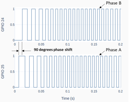
An encoder or, more specifically, a rotary incremental encoder is a device that can be used to determine incremental changes of the angular position of a rotating shaft. One of the possible hardware constructions is based on a slotted disk attached to the shaft and a pair of optical sensors with a physical offset. The detection of “dark/bright” transitions, as the shaft rotates and the slots pass in front of the sensors, is converted by an electronic circuit into two pulse trains that have a phase shift of 90 degrees between them.
The two signals that are generated by the encoder have to be then processed by a DAQ device, so that the angular increment (or decrement) of the shaft can be determined by “counting the high/low edge transitions” of the two signals. Some DAQ devices have a hardware implementation to deal with encoder signals, thus allowing for much higher shaft speeds. As it is the case of a LabJack.
The Raspberry Pi, on the other hand, doesn’t have the capability to deal with pulse train inputs via hardware. Therefore, it has to rely on a software implementation to do the “edge counting”. We will focus on the class RotaryEncoder in GPIO Zero, which is quite good and very straightforward to use.
To follow along the contents of this post, you may want to review my previous post (H-Bridge and DC Motor with Raspberry Pi), since a motor with an integrated encoder will be used in the examples and, by the end, we will expand the Motor class by adding encoder input capability to it.
From a nomenclature stand point, encoders that produce a pair of square waves (pulse trains) with a 90-degree phase shift are also known as quadrature encoders. However, to take full advantage of this type of encoder, i.e., count all 4 edge transitions during the rotation through one marker (or slot), a hardware-based edge detection is usually required. So, an encoder disc with 45 slots would give a count of 180 effective pulses per revolution (PPR) for a resolution of 2 degrees (360/180). When using a software-based edge detection, the same encoder would have 45 PPR and a resolution of 8 degrees.
The figure below shows typical connections for a Raspberry Pi. Note that the A and B phases are interchangeable. If the pulse count is decreasing when you’re expecting a positive rotation, just swap the connections of the phase wires.

Checking the PPR of the Encoder
After the encoder is connected to the Pi, as shown above, you can use the following Python code to check if the number of Pulses Per Revolution is what you’re expecting. A couple of things will factor into the PPR value.
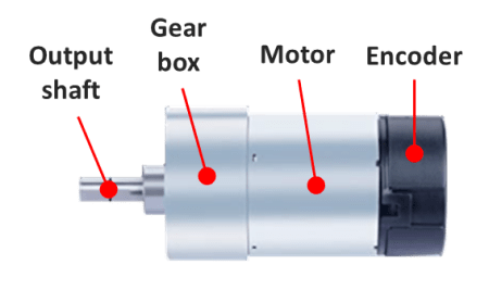
If the motor has a gear box, the “advertised” PPR value might be incorrect. First of all, understand if the number refers to the quadrature-based value or the marker-based value. Then check if the number is taking into account the gear ratio of the box.
In my case, I am using a motor with a 16 PPR encoder (advertised as a 64 based on a full quadrature implementation) and a gear ratio of 18.8:1. That gives a value of 16 x 18.8 = 300.8 PPR. Ultimately, you can use the sample program below and turn the output shaft by hand to see what you get!
# Importing modules and classes
import time
import numpy as np
from gpiozero import RotaryEncoder

# Assigning parameter values
ppr = 300.8  # Pulses Per Revolution of the encoder
tstop = 20  # Loop execution duration (s)
tsample = 0.02  # Sampling period for code execution (s)
tdisp = 0.5  # Sampling period for values display (s)

# Creating encoder object using GPIO pins 24 and 25
encoder = RotaryEncoder(24, 25, max_steps=0)

# Initializing previous values and starting main clock
anglecurr = 0
tprev = 0
tcurr = 0
tstart = time.perf_counter()

# Execution loop that displays the current
# angular position of the encoder shaft
print('Running code for', tstop, 'seconds ...')
print('(Turn the encoder.)')
while tcurr <= tstop:
    # Pausing for `tsample` to give CPU time to process encoder signal
    time.sleep(tsample)
    # Getting current time (s)
    tcurr = time.perf_counter() - tstart
    # Getting angular position of the encoder
    # roughly every `tsample` seconds (deg.)
    anglecurr = 360 / ppr * encoder.steps
    # Printing angular position every `tdisp` seconds
    if (np.floor(tcurr/tdisp) - np.floor(tprev/tdisp)) == 1:
        print("Angle = {:0.0f} deg".format(anglecurr))
    # Updating previous values
    tprev = tcurr

print('Done.')
# Releasing GPIO pins
encoder.close()
Motor Class with Encoder
The following diagram expands upon the motor setup from the post (H-Bridge and DC Motor with Raspberry Pi). Just as before, we’re using the SN754410 half-bridge chip to set the motor output. But this time around, we can use the encoder to measure the actual shaft angular position and speed.

The Motor class from the post mentioned above can be updated by doing a few modifications to incorporate the rotary encoder.
Besides some new attributes (or properties) used to handle the encoder parameters and its object, two new methods were added: get_angle(), which returns the current encoder angular position in degrees, and reset_angle(), which resets the encoder angle to zero (a handy functionality to have, since we’re using an incremental encoder).
The updated and fully commented class, as well as the rest of the code in this post, can be found on my GitHub page. Also, if you haven’t done it already, I strongly encourage installing VS Code on Raspberry Pi.
Sinusoidal Motor Excitation
The Python program below uses the updated Motor class to run the DC motor with a sinusoidal excitation. Now that we have the encoder capability added to the class, it is possible to measure the angular position of the shaft and calculate its angular velocity. If you’re using VS Code, you must run the code in a terminal instead of an interactive window. The interactive session really competes with the code for CPU resources.
# Importing modules and classes
import time
import numpy as np
from utils import plot_line
from gpiozero_extended import Motor

# Assigning parameter values
T = 2  # Period of sine wave (s)
u0 = 1  # Motor output amplitude
tstop = 2  # Sine wave duration (s)
tsample = 0.01  # Sampling period for code execution (s)

# Creating motor object using GPIO pins 16, 17, and 18
# (using SN754410 quadruple half-H driver chip)
# Integrated encoder is on GPIO pins 25 and 25
mymotor = Motor(
    enable1=16, pwm1=17, pwm2=18,
    encoder1=24, encoder2=25, encoderppr=300.8)
mymotor.reset_angle()

# Pre-allocating output arrays
t = []
theta = []

# Initializing current time step and starting clock
tprev = 0
tcurr = 0
tstart = time.perf_counter()

# Running motor sine wave output
print('Running code for', tstop, 'seconds ...')
while tcurr <= tstop:
    # Pausing for `tsample` to give CPU time to process encoder signal
    time.sleep(tsample)
    # Getting current time (s)
    tcurr = time.perf_counter() - tstart
    # Assigning motor sinusoidal output using the current time step
    mymotor.set_output(u0 * np.sin((2*np.pi/T) * tcurr))
    # Updating output arrays
    t.append(tcurr)
    theta.append(mymotor.get_angle())
    # Updating previous time value
    tprev = tcurr

print('Done.')
# Stopping motor and releasing GPIO pins
mymotor.set_output(0, brake=True)
del mymotor

# Calculating motor angular velocity (rpm)
w = 60/360 * np.gradient(theta, t)

# Plotting results
plot_line([t, t, t[1::]], [theta, w, 1000*np.diff(t)], axes='multi',
          yname=[
              'Angular Position (deg.)',
              'Angular velocity (rpm)',
              'Sampling Period (ms)'])
Once the code finishes running you should get the graph on the bottom left in a web browser page, assuming you ran it in a VS Code terminal. Differently from my other execution loops, I force an execution “pause” by using the command time.sleep(tsample) inside the loop.

By taking that approach, at the expense of a more accurate sampling period, I free up kernel resources to process other interruptions, such as the very CPU-intensive ones coming from the RotaryEncoder. The object is now capable of detecting all the edge transitions coming from the physical encoder, minimizing the number of missed events.
Taking a closer look at the derivative of the angular position (or the velocity) we can detect some fluctuations that are probably due to missed edge counts. The faster the shaft turns, the more likely that is to happen. In our case, 300 PPR at 400 rpm gives 300 x 400 / 60 = 2000 pulses per second. And because the algorithm inside the RotaryEncoder class has to detect all four edge transitions within a pulse, that puts us at 8000 events/sec (or 125 μs/event). Even though the computer is running individual calculations at the nanosecond level, there are many calculations going on inside the algorithm alongside other synchronous tasks. So 125 μs is probably cutting it close.
Still analyzing the results, the sinusoidal PWM excitation will roughly produce a sinusoidal current input to the motor. Since it is the torque, not the angular velocity, that is proportional to the input current, the speed trace will deviate somewhat from the shape of an actual sine wave. That is also quite apparent on the angular position trace, which should be a cosine wave. The deviations with respect to the expected trace shapes are caused mainly by torque being consumed to overcome friction losses in the initial motion and the response time of the motor itself, as a dynamic system.
That is the inherent behavior of this open-loop system. Now that we have the elements in place, by adding the capability to measure the system output, in future posts we’ll explore what can be done by closing the loop on the angular position of the motor shaft.
