Robots that can follow a line on the floor (more specifically AGVs – Automated Guided Vehicles) have been around for quite some time now, moving around in factories and warehouses. The most basic ones follow a magnetic embedded tape or an actual line painted on the floor. In this post, we will take a closer look at a sensor whose output is a continuous value that can be used with the Raspberry Pi. There are quite a few so-called line tracking sensors available for the Pi. However, most of them provide a digital output, i.e., they detect whether you are either on (one) or off (zero) the line, putting the burden on the control system that has to deal with only two possible sensor states. A sensor with a continuous output is much more suitable for what is primarily a set-point tracking control problem.
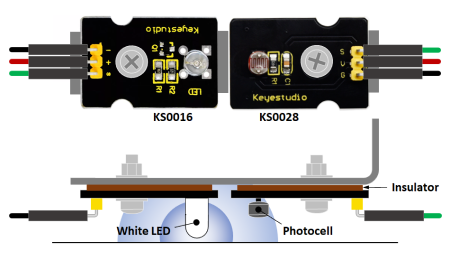
The pictorial representation on the left shows the two electronic components that were used to make the sensor: a white LED (Keyestudio KS0016) and a photocell (KS0028). The former provides a consistent light source and the latter senses the reflected light intensity off the surface the sensor is pointing at.
In you are mounting the two components to a metal bracket, it is VERY IMPORTANT to use an insulator as shown in the picture! Otherwise, you will short the soldered tips on the circuit boards and permanently damage your Raspberry Pi. I used the paper from a cereal box, folded to the desired thickness.
The wiring schematic below shows how the LED and the photocell are integrated with the Raspberry Pi. Since the photocell output is continuous, an MCP3008 analog-to-digital converter chip is also required.
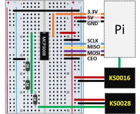
The connection of the LED to the Pi is pretty straightforward, with the signal pin connected to a GPIO pin of your choosing. In my case, I went with pin 18.
Taking a closer look at the MCP3008 connections, I used 3.3V as the reference voltage for the chip (instead of 5V) for a better absolute resolution.
Since both components require a 5V supply voltage, for the KS0028, a voltage divider must be used to bring the maximum photocell output down to 3.3V (or less) before connecting it to the MCP3008. After doing some testing, a 1 kΩ / 4 kΩ split gave me the ratio that best utilized the 3.3V range.
Sensor Characterization
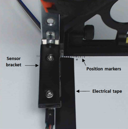
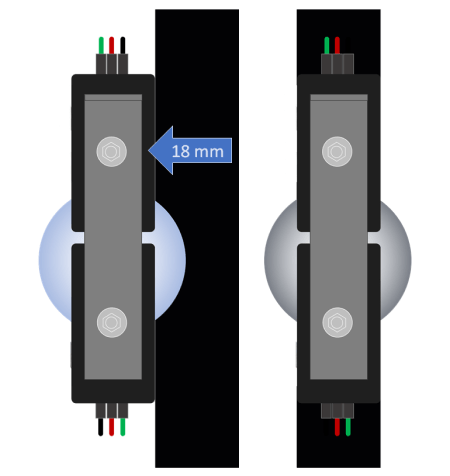
The actual sensor setup is shown next, where I used black electrical tape (approx. 18 mm wide) as the line to be followed. The test procedure for the sensor characterization is illustrated on the right at its initial position (marker 0 on the actual sensor picture) and final position (after moving the bracket in 2 mm steps until reaching 18 mm). As a side note, the LED tip sits at approximately 5 mm above the surface.
The table below shows the normalized sensor output (where 1 would be the reference voltage of 3.3V) for three sets of measurements at 2 mm position increments. Observe that the row at 18 mm was omitted, since its values were basically the same as the row at 16 mm. That means that the sensor was already being exposed to the maximum amount of reflected light off the white surface at 16 mm. Additionally, the sensor placed fully above the black line (position 0) gives the lowest output for the reflected light, which is about 0.43.
| Position (mm) | Output Meas. 1 | Output Meas. 2 | Output Meas. 3 | Mean Output |
|---|---|---|---|---|
| 0 | 0.438 | 0.432 | 0.427 | 0.432 |
| 2 | 0.450 | 0.449 | 0.444 | 0.448 |
| 4 | 0.494 | 0.448 | 0.450 | 0.477 |
| 6 | 0.548 | 0.544 | 0.548 | 0.547 |
| 8 | 0.654 | 0.638 | 0.668 | 0.653 |
| 10 | 0.807 | 0.790 | 0.804 | 0.800 |
| 12 | 0.915 | 0.905 | 0.904 | 0.908 |
| 14 | 0.933 | 0.934 | 0.931 | 0.933 |
| 16 | 0.948 | 0.957 | 0.960 | 0.955 |
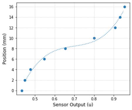
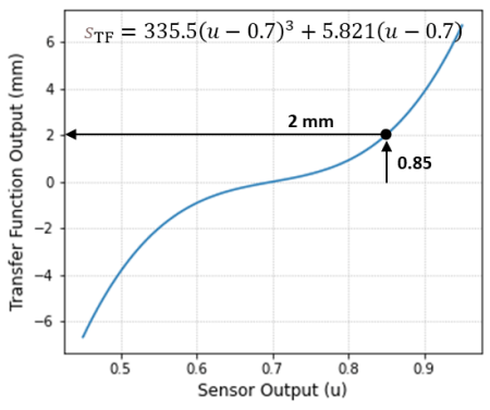
The plot on the left shows the bracket position as a function of the sensor output and the fitted cubic polynomial. The plot on the right shows the transfer function that characterizes the sensor, which is basically the fitted polynomial with the appropriate shift and offset.
A few notes on the transfer function:
- Technically speaking, the sensor transfer function provides the relationship between the physical input (position, in this case) and the sensor output (normalized voltage). In this particular post, I will be calling that one “sensor output function“. The relationship between sensor output and physical input that is to be implemented in code will then be called transfer function.
- The variability on the sensor output is more likely due to the variability of the position, since eyeballing the exact 2 mm steps when moving the bracket has plenty of uncertainty to it.
- The transfer function is basically the inverse of the physical sensor output function and would reside inside the software bridging the real world and the control system. Moreover, it linearizes the sensor behavior! For example, if the bracket is at the position 2 mm, the sensor output would be 0.85. However, once that measurement is brought into the control software and input into the transfer function, the output is an estimation of the original position of 2 mm.
The Python code below was used to generate the previous plots and determine the coefficients for the transfer function. The next section shows some polynomial trickery used to calculate the shift and offset for the fitted cubic function, centered around the position at which the LED is right on the transition between the white and black surfaces (the inflection at 0.7).
# Importing modules and classes
import numpy as np
import matplotlib.pyplot as plt
from numpy.polynomial import Polynomial as P

# Defining function to generate Matplotlib figure with axes
def make_fig():
    #
    # Creating figure
    fig = plt.figure(
        figsize=(5, 4.2),
        facecolor='#ffffff',
        tight_layout=True)
    # Adding and configuring axes
    ax = fig.add_subplot(
        facecolor='#ffffff',
        )
    ax.grid(
    linestyle=':',
    )
    # Returning axes handle
    return ax


# Defining data values u (sensor output) and s (bracket position)
# from sensor characterization test
u = [0.432, 0.448, 0.477, 0.547, 0.653, 0.800, 0.908, 0.933, 0.955]
s = [0, 2, 4, 6, 8, 10, 12, 14, 16]

# Fitting 3rd order polynomial to the data
p, stats = P.fit(u, s, 3, full=True)
# Evaluating polynomial for plotting
ui = np.linspace(0.45, 0.95, 100)
si = p(ui)
# Plotting data and fitted polynomial
ax = make_fig()
ax.set_xlabel('Sensor Output (u)', fontsize=12)
ax.set_ylabel('Position (mm)', fontsize=12)
ax.scatter(u, s)
ax.plot(ui, si, linestyle=':')

# Getting polynomial coefficients
c = p.convert().coef
# Calculating coefficients for transfer function
# (shift and offset representation)
k = c[3]
u0 = -c[2]/(3*k)
w = c[1] - 3*k*u0**2
s0 = c[0] + k*u0**3 + w*u0
# Defining transfer function for plotting
stf = k*(ui-u0)**3 + w*(ui-u0)
# Plotting transfer function
ax = make_fig()
ax.set_xlabel('Sensor Output (u)', fontsize=12)
ax.set_ylabel('Transfer Function Output (mm)', fontsize=12)
ax.plot(ui, stf)

# Calculating root mean squared error from residual sum of squares
rss = stats[0]
rmse = np.sqrt(rss[0]/len(s))
# Calculating R-square
r2 = 1 - rss[0]/np.sum((s-np.mean(s))**2)
# Displaying fit info
print('R-square = {:1.3f}'.format(r2))
print('RMSE (mm) = {:1.3f}'.format(rmse))
print('')
print('Shift (-) = {:1.3f}, Offset (mm) = {:1.3f}'.format(u0, s0))
Polynomial Trickery
Let’s see how we can determine the shift and offset of a third order polynomial that is expressed in its most general form:

Due to the nature of the sensor response, it is reasonable to assume that the corresponding polynomial in its shift and offset form is odd (other than the offset term) and can be expressed as:

Both representations have 4 coefficients that need to be determined (![]() or
or![]() ). The polynomial fitting gave us the first set, so we need to determine
). The polynomial fitting gave us the first set, so we need to determine![]() as a function of
as a function of![]() . To do so, let’s expand the second polynomial above and regroup its terms in descending powers of x:
. To do so, let’s expand the second polynomial above and regroup its terms in descending powers of x:

Finally, all we have to do is equate (solving for the variables of interest) the corresponding coefficients of the polynomial above with the one at the top of this section:

Which is exactly what’s in the Python code that produced the transfer function for the line tracking sensor.
Sensor Python Class
From a control software standpoint, the best way to use the line tracking sensor with a robot is to package its transfer function inside a class. That way, it’s much easier to get the sensor position reading within a control loop. The Python code below contains the LineSensor class, in which the transfer function can be easily identified. The motor speed control post can be a starting point for a closed-loop control using the PID class. That one and a more complete version of LineSensor can be found in gpiozero_extended.py.
# Importing modules and classes
import time
import numpy as np
from gpiozero import MCP3008, DigitalOutputDevice

class LineSensor:
    """
    Class that implements a line tracking sensor.

    """
    def __init__(self, lightsource, photosensor):
        # Defining transfer function parameters
        self._k = 335.5
        self._w = 5.821
        self._u0 = 0.700
        # Creating GPIOZero objects
        self._lightsource = DigitalOutputDevice(lightsource)
        self._photosensor = MCP3008(
            channel=photosensor,
            clock_pin=11, mosi_pin=10, miso_pin=9, select_pin=8)
        # Turning light source on
        self._lightsource.value = 1

    @property
    def position(self):
        # Getting sensor output
        u = self._photosensor.value
        # Calculating position using transfer function
        return self._k*(u-self._u0)**3 + self._w*(u-self._u0)

    @position.setter
    def position(self, _):
        print('"position" is a read only attribute.')

    def __del__(self):
        self._lightsource.close()
        self._photosensor.close()


# Assigning some parameters
tsample = 0.1  # Sampling period for code execution (s)
tdisp = 0.5  # Output display period (s)
tstop = 60  # Total execution time (s)
# Creating line tracking sensor object on GPIO pin 18 for
# light source and MCP3008 channel 0 for photocell output
linesensor = LineSensor(lightsource=18, photosensor=0)

# Initializing variables and starting main clock
tprev = 0
tcurr = 0
tstart = time.perf_counter()
# Execution loop
print('Running code for', tstop, 'seconds ...')
while tcurr <= tstop:
    # Getting current time (s)
    tcurr = time.perf_counter() - tstart
    # Doing I/O and computations every `tsample` seconds
    if (np.floor(tcurr/tsample) - np.floor(tprev/tsample)) == 1:
        # Getting sensor position
        poscurr = linesensor.position
        #
        # Insert control action here using gpiozero_extended.PID()
        #
        # Displaying sensor position every `tdisp` seconds
        if (np.floor(tcurr/tdisp) - np.floor(tprev/tdisp)) == 1:
            print("Position = {:0.1f} mm".format(poscurr))
    # Updating previous time value
    tprev = tcurr

print('Done.')
# Deleting sensor
del linesensor
Final Remarks
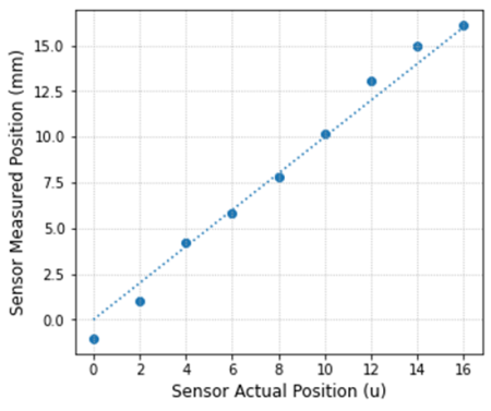
First, it’s important to check how well the transfer function estimates the actual position of the sensor. That can be done by running the code from the previous section placing the bracket at the original test positions.
The graph on the left shows measured values (from the code output) vs. desired values (by moving the bracket onto each test marker). The dashed line represents the 45-degree line on which measured values match actual ones. You can find the code for it here.
The error is more accentuated away from the center, which seems to be where the cubic fit deviates more from the test points.
Second, the ambient light intensity does affect the sensor reading and therefore will compromise the validity of the transfer function. It is important then to determine the transfer function with lighting conditions that represent where the robot will be running. Preferably, with the sensor mounted on the robot!
Finally, for this specific sensor, the width of the line should be about 20 mm. If the line is too thin, or if the robot is moving too fast for the turn it’s supposed to make, the position deviation may exceed the line thickness. In that case, the sensor would again be “seeing” a white surface on the wrong side of the line(!), causing the negative feedback loop of the control system to become a positive one, moving the robot further away from the line.

One thought on “Line Tracking Sensor for Raspberry Pi”