Let’s use the Motor class with encoder and the Digital PID class to create a closed-loop speed controller for a DC motor. Those two classes have all the required attributes and methods that we need to program an execution loop for a PID controller with very few lines of code.

The starting point is the Raspberry Pi setup that was used to implement encoder capability into the Motor class. I took the artistic liberty to create the diagram below, where I combine visual elements of the PID loop, the hardware connections, and the class methods used for the I/O between the Pi computer and the physical system.

Going back to the concept of execution loops, the I/O tasks are taken care by the Motor class methods get_angle() and set_output(). The computation tasks happening in between are essentially the shaft speed calculation, low-pass filtering, and PID control action. The Python code below implements the execution loop, where the different elements in the Pi box above can be identified. The complete program, which includes the plotting features, along with the Python module with all necessary classes, can be found on my GitHub page.

# Importing modules and classes
import time
import numpy as np
from gpiozero_extended import Motor, PID

# Setting general parameters
tstop = 2  # Execution duration (s)
tsample = 0.01  # Sampling period (s)
wsp = 20  # Motor speed set point (rad/s)
tau = 0.1  # Speed low-pass filter response time (s)

# Creating PID controller object
kp = 0.15
ki = 0.35
kd = 0.01
taupid=0.01
pid = PID(tsample, kp, ki, kd, umin=0, tau=taupid)

# Creating motor object using GPIO pins 16, 17, and 18
# (using SN754410 quadruple half-H driver chip)
# Integrated encoder on GPIO pins 24 and 25.
mymotor = Motor(
    enable1=16, pwm1=17, pwm2=18,
    encoder1=24, encoder2=25, encoderppr=300.8)
mymotor.reset_angle()

# Initializing previous and current values
ucurr = 0  # x[n] (step input)
wfprev = 0  # y[n-1]
wfcurr = 0  # y[n]

# Initializing variables and starting clock
thetaprev = 0
tprev = 0
tcurr = 0
tstart = time.perf_counter()

# Running execution loop
print('Running code for', tstop, 'seconds ...')
while tcurr <= tstop:
    # Pausing for `tsample` to give CPU time to process encoder signal
    time.sleep(tsample)
    # Getting current time (s)
    tcurr = time.perf_counter() - tstart
    # Getting motor shaft angular position: I/O (data in)
    thetacurr = mymotor.get_angle()
    # Calculating motor speed (rad/s)
    wcurr = np.pi/180 * (thetacurr-thetaprev)/(tcurr-tprev)
    # Filtering motor speed signal
    wfcurr = tau/(tau+tsample)*wfprev + tsample/(tau+tsample)*wcurr
    wfprev = wfcurr
    # Calculating closed-loop output
    ucurr = pid.control(wsp, wfcurr)
    # Assigning motor output: I/O (data out)
    mymotor.set_output(ucurr)
    # Updating previous values
    thetaprev = thetacurr
    tprev = tcurr

print('Done.')
# Stopping motor and releasing GPIO pins
mymotor.set_output(0, brake=True)
del mymotor

Motor Speed Filtering

Now that the Python code is laid out, let’s go over some of its components. The motor shaft speed is calculated as the derivative of the angular position of the shaft using a backward difference formula wcurr = np.pi/180 * (thetacurr-thetaprev)/(tcurr-tprev).

The encoder that’s being used has a resolution of encoderppr=300.8, which corresponds to approximately 360/300.8 = 1.2 degrees. The difference between two consecutive time steps tcurr and tprev is about tsample = 0.01 seconds. That gives us a not so great speed resolution of np.pi/180 * (1.2)/(0.01) = 2 rad/s (or 19 rpm!). As a side note, the speed resolution could be improved by increasing either the encoder PPR or the sampling rate. However the first option might reach the limit of the GPIO zero RotaryEncoder class, while the latter will eventually make the closed-loop system unstable. Therefore a compromise has to be reached given the constraints at hand.

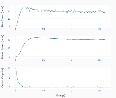
One way reduce the impact of this limitation is to apply a low-pass digital filter to the motor speed signal: wfcurr = tau/(tau+tsample)*wfprev + tsample/(tau+tsample)*wcurr. The graphs below show the raw and the filtered signal as well as the controller output.

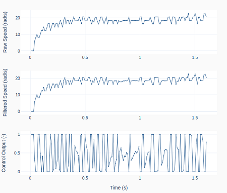
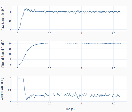
On the left, tau = 0 and therefore no filtering is being done. Observe how the controller output bounces between saturation limits. On the right, tau = 0.1, causing the control output to be less erratic, which in turn makes the raw speed more stable. One can also see the “discretization effect” of the 2 rad/s speed resolution on the top row plots.

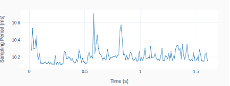
As discussed in the post Encoder with Raspberry Pi, we cannot use a more accurate sampling period during the execution loop due to the intensive computing resources of the RotaryEncoder class.

However, as shown on the left, having to rely on the command time.sleep(tsample) inside the execution loop, still produces repeatability of the sampling period within 1 ms.

PID Derivative Term Filtering

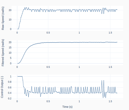
If you notice in the Python code above, I am also filtering the PID derivative when I created the PID class instance: pid = PID(tsample, kp, ki, kd, umin=0, tau=taupid), where taupid = 0.01 seconds.

If we turn it off by making taupid = 0, we obtain the results on the left, where the controller output shows a bigger oscillation amplitude. However, the effect of turning the derivative term filter off is not as pronounced as the effect of not filtering the motor speed signal.

By comparing all the system responses so far, even though the PID gains were never changed from case to case, the closed-loop system response is changing. Ultimately, by adding low-pass filters, the closed-loop dynamic system is different from its original form without the filters.

PID Saturation and Anti-Windup

As it can be seen in the previous graphs, the PID output is saturating right after the step input. We can observe the effect of PID saturation and the integral term windup (which has been avoided so far) by creating the PID class instance: pid = PID(tsample, kp, ki, kd, umin=-10, umax=10, tau=taupid).

Because the controller output (PWM in the Motor class) is in fact limited between -1 and 1, applying -10 and 10 as the new PID controller limits will effectively turn off the anti-windup feature and cause the integral term to wind up.

The plots on the left show the resulting speed overshoot due to that modification as the actual PWM output is saturated at 1.

Final Remarks

We have been building up our knowledge with the previous posts (namely: Encoder with Raspberry Pi, Digital Filtering, and Digital PID Controller) so we could finally run a DC motor in closed-loop speed control. While this could have been achieved from the very beginning, I believe it was more educational to do it in smaller parts through the use of Python classes.

When building more complex automation systems, having a modularized approach with classes that can be tested and used independently, as well as combined in different ways, will make things much easier to tackle in the long run.

• Automation
• Engineering