At the end of the post Motor Position Control with Raspberry Pi, we saw that there are different ways to move a motor shaft between two angular positions. In this post, we will take a deeper look into three types of paths between an initial and a final position. While I’ll be exploring the concept using a system with one degree of freedom, with proper normalization and parametrization, the idea can be applied to any trajectory between two points in space.
The first observation to be made is that the path that our closed-loop system is going to follow is calculated before hand, i.e., the initial and final positions![]() and
and![]() (shown in the diagram on the left), as well as other parameters that define the trajectory, are known before the position tracking is executed.
(shown in the diagram on the left), as well as other parameters that define the trajectory, are known before the position tracking is executed.
In our case, we’ll use the acceleration time![]() (at the beginning and end of the motion) and the maximum allowed velocity
(at the beginning and end of the motion) and the maximum allowed velocity![]() as the additional parameters that are sufficient to fully determine the path.
as the additional parameters that are sufficient to fully determine the path.
Maximum velocity and acceleration time (or conversely the maximum acceleration) are a reasonable choice, since they are related to the physical limitations of the system.
The total motion time is therefore automatically determined once the four parameters above are specified. Even though there are different ways to go about calculating the path, I’ll use the velocity profile as the primary trace, with position and acceleration being calculated respectively as the integral and derivative of the velocity. Let’s then go over the three velocity profiles for this post: linear, quadratic, and trigonometric.
Linear Speed Profile
Using the illustration below it’s not too difficult to arrive at the following three equations that describe the velocity as a function of time.
The time![]() at maximum speed is given by:
at maximum speed is given by:
Where it can be calculated by using the fact that the area under the speed trace is equal to ![]() .
.
As mentioned before, ![]() and
and ![]() can be used interchangeably, where, in this case,
can be used interchangeably, where, in this case, ![]() . The Python function below shows one possible implementation of the path calculation, where the position and acceleration traces are calculated through numerical integration and derivative, respectively. I found this approach to be more robust to the path discretization, specially at the speed profile transitions.
. The Python function below shows one possible implementation of the path calculation, where the position and acceleration traces are calculated through numerical integration and derivative, respectively. I found this approach to be more robust to the path discretization, specially at the speed profile transitions.
def path_linear(xstart, xstop, vmax, ta, nstep=1000):
    #
    # Adjusting velocity based on end points
    if xstop < xstart:
        vmax = -vmax
    # Assigning time at max velocity
    if (xstop-xstart)/vmax > ta:
        # There's enough time for constant velocity section
        tmax = (xstop-xstart)/vmax - ta
    else:
        # There isn't (triangular velocity profile)
        tmax = 0
        vmax = (xstop-xstart)/ta
    # Assigning important time stamps
    t1 = ta  # End of acceleration section
    t2 = ta + tmax  # End of constant velocity section
    t3 = 2*ta + tmax  # End of motion (deceleration) section
    # Creating time array for path discretization
    t = np.linspace(0, t3, nstep+1)
    # Finding transition indices
    i1 = np.nonzero(t<=t1)
    i2 = np.nonzero((t>t1)&(t<=t2))
    i3 = np.nonzero(t>t2)
    # Calculating accelereration section array
    v1 = vmax/ta*t[i1]
    # Calculating constant velocity section array
    if len(i2[0]) > 0:
        v2 = np.array([vmax]*len(i2[0]))
    else:
        v2 = np.array([])
    # Calculating deceleration section array
    v3 = vmax - vmax/ta*(t[i3]-t2)
    # Concatenating arrays
    v = np.concatenate((v1, v2, v3))
    # Calculating numeric integral (position)
    x = xstart + t[-1]/nstep * np.cumsum(v)
    # Calculating numeric derivative (acceleration)
    a = np.gradient(v, t)
    # Returning time, position, velocity, and acceleration arrays
    return t, x, v, a
Quadratic Speed Profile
Unlike the linear speed profile, which uses constant acceleration, the quadratic (or parabolic) speed profile uses linearly changing acceleration at the beginning and end of the motion. The equations for this type of trajectory are shown below.
An easy way to obtain the first and third velocity equations above is by writing the corresponding acceleration functions and integrating them.
Similarly to the linear case, the time at maximum speed can be obtained from the area under the velocity curve. (Tip: integrate the first velocity equation and evaluate it at![]() , multiply the result by 2 to account for the deceleration portion, and add the area of the rectangle under
, multiply the result by 2 to account for the deceleration portion, and add the area of the rectangle under![]() )
)
The Python function for this case follows the same structure as the previous one. You can find it on my GitHub page.
Trigonometric Speed Profile
The third profile type uses a cosine function for the velocity during the acceleration and deceleration phases of the trajectory. By choosing the appropriate function, it is possible to add an interesting feature to this last profile type: zero initial and final accelerations.
Also through integration of the velocity function and knowing that the area under the curve is![]() , it is possible to solve for the time at maximum velocity:
, it is possible to solve for the time at maximum velocity:
Like the two previous cases, the Python function that implements this type of path calculation is located on the GitHub page.
Practical Application for Position Tracking
When it comes to choosing the path calculation method, two factors have to be kept in mind: how fast do we want to (or can) go from the initial to the final position and how much acceleration change (jerk) do we want to apply to the system. One good way to go about it is to test all three and quantify how the overall closed-loop system behaves.
Just to explore a little bit, the plot on the left shows an overlay of the three types of path for the examples shown above. In this scenario, the maximum velocity is limited to 1 (m/s, for example) and the total time set to 1.4s, by proper choice of![]() . Even though the acceleration profiles are very distinct, the difference between the three types of trajectory is visually very subtle.
. Even though the acceleration profiles are very distinct, the difference between the three types of trajectory is visually very subtle.
In contrast, if we now limit both the maximum velocity to 1 m/s and the maximum acceleration to 4 m/s2, the total motion duration is fairly different. The linear velocity profile is the fastest one (at the expense of having the largest jerk). Conversely, the trigonometric method takes the longest time with the least amount of jerk.
Let’s use the same setup with a Raspberry Pi and a DC motor that we had in the post Motor Position Control with Raspberry Pi to test the different types of paths for the positioning of the DC motor shaft. The Python program below shows how the quadratic path is generated prior to the execution loop and then sampled during the execution loop.
The full code with the plotting features and the module path.py, containing the three types of path calculation functions, can be found here.
# Importing modules and classes
import time
import numpy as np
from scipy.interpolate import interp1d
from path import path_quad
from gpiozero_extended import Motor, PID
# Setting path parameters
thetastart = 0 # Start shaft angle (rad)
thetaend = 3*np.pi # End shaft angle (rad)
wmax = 4*np.pi # Max angular speed (rad/s)
ta = 0.45 # Acceleration time (s)
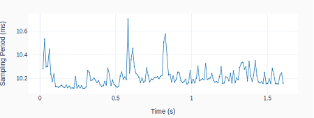
tsample = 0.01 # Sampling period (s)
# Calculating path
t, x, _, _ = path_quad(thetastart, thetaend, wmax, ta)
f = interp1d(t, 180/np.pi*x) # Interpolation function
tstop = t[-1] # Execution duration (s)
# Creating PID controller object
kp = 0.036
ki = 0.260
kd = 0.0011
taupid = 0.01
pid = PID(tsample, kp, ki, kd, tau=taupid)
# Creating motor object using GPIO pins 16, 17, and 18
# (using SN754410 quadruple half-H driver chip)
# Integrated encoder on GPIO pins 24 and 25.
mymotor = Motor(
enable1=16, pwm1=17, pwm2=18,
encoder1=24, encoder2=25, encoderppr=300.8)
mymotor.reset_angle()
# Initializing variables and starting clock
thetaprev = 0
tprev = 0
tcurr = 0
tstart = time.perf_counter()
# Running execution loop
print('Running code for', tstop, 'seconds ...')
while tcurr <= tstop:
# Pausing for `tsample` to give CPU time to process encoder signal
time.sleep(tsample)
# Getting current time (s)
tcurr = time.perf_counter() - tstart
# Getting motor shaft angular position
thetacurr = mymotor.get_angle()
# Interpolating set point angle at current time step
if tcurr <= tstop:
thetaspcurr = f(tcurr)
# Calculating closed-loop output
ucurr = pid.control(thetaspcurr, thetacurr)
# Assigning motor output
mymotor.set_output(ucurr)
# Updating previous values
thetaprev = thetacurr
tprev = tcurr
print('Done.')
# Stopping motor and releasing GPIO pins
mymotor.set_output(0, brake=True)
del mymotor
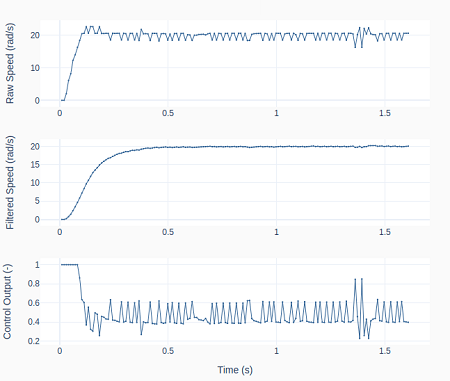
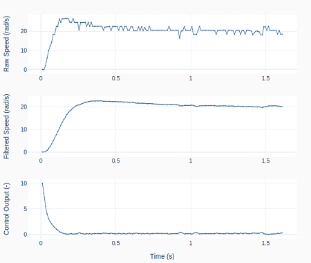
The plots show the set point vs. actual shaft position for a 450 degrees rotation, using the quadratic velocity path.
The derivative of the signal, i.e., the shaft speed, is a useful gage to see how well the closed-loop system can follow the trajectory. The position error between set point and measured value is also a good metric. In this case, it is within +/- 5 degrees with an RMSE (Root Mean Squared Error) of about 2.5 degrees. Although not a stellar result, it’s not too bad, given the budget hardware and simple control (PID) that were used.
Finally, the graph at the bottom shows a comparison of the position tracking error for the three types of path explored in this post for the same 450 degree rotation. The average RMSE values for the linear, quadratic, and trigonometric speed profiles were respectively 3.3, 2.4, and 3.6 degrees.
Even though the trigonometric profile has the smoothest acceleration, it was outperformed by the other two for this particular system.
The trigonometric one is usually beneficial for dynamic systems that are more susceptible to vibration when subjected to a more “jerky” path profile.