Tag: DAQ

Circular Buffer in Python

Circular Buffer in Python

A circular or ring buffer is a fixed-size data structure that is commonly used in real-time software applications to store a pre-defined number of values. The analogy of a ring with a fixed number of positions is quite useful to capture the FIFO (First-In-First-Out) nature of such data structure. Once the buffer is full, the first element that was written (“In” ) to the buffer is the first one to be overwritten (“Out”) by the next incoming element.

Circular buffers are particularly useful in situations where the data is continuously being sampled and calculations need to be done using a pre-defined sample size or continuous visualization is required.

The two images below represent a circular buffer with 10 positions. On the left, with four elements written to it being 5 the “first in”. On the right, the buffer is full where the value 3 was written. Note how the current write position pointer moves around as new values are added.

Additionally, a ring buffer has basically two states: not-yet- full (left image) and full (right image). The not-yet-full state occurs after the buffer is initialized and exists only until it becomes full. We will see later how this affects the Python code used to represent the buffer.

Once the buffer state changes to full, the FIFO nature of this type of data structure becomes evident. In the next two images, the next element “in” is the value 12, replacing the “first in” value 5, which therefore is the “first out”. The next value “in” is 2, replacing the “second in” value 10, and so on.

In the example figures above, we could imagine the buffer being used to display the average value of its elements (once the buffer reaches the full state). As time progresses, a new sample is written to the buffer, replacing the oldest sample. Each figure of the full buffer is a snapshot at a given time step of the sampling process. In this case the average values are 6.4, 7.1, and 6.3.

Python Implementation

The most elegant way to implement the circular buffer is by using a class. Also, a true circular buffer does not involve shifting its elements to implement the FIFO structure. The current position pointer is used to keep track of where the newest element is.

The circular buffer class should have the following attributes:

  • bufsize: the number of elements that the circular buffer can hold (integer)
  • data: the list of elements, i.e., the buffer itself
  • currpos: the current position pointer (integer)

The class should also have two methods:

  • add(): writes an element to the buffer
  • get(): returns a list containing the buffer elements

Let’s go over some of the features of the Python implementation below:

  • As mentioned earlier, the ring buffer has two states (not-yet-full and full). The first state only exists for a limited time until the buffer is filled up. With that in mind, it makes sense to define the __Full class within the RingBuffer class with the exact same methods. Once the buffer is full, the original class is permanently changed to the full class implementation, with its add() and get() methods now superseding the original ones.
  • The not-yet-full add() method just does a regular list append operation of new elements to the buffer list. It is also in this method that the class is changed to the __Full class once the buffer reaches its capacity.
  • The full add() method, on the other hand, writes the new element at the current (newest) element position and increments the current position by one unit (wrapping it around, or resetting it, once the buffer size value is reached).
  • More interesting however is the full get() method. It splits the data list at the current position into two lists which are then concatenated. The list going from currpos to the last element goes first, then comes the list from the first element to currpos (excluded). By returning this concatenated list, the method fully implements the circular buffer without shifting any of it elements! Inspect the data attribute as you add elements to a full buffer to see what the original list looks like.
class RingBuffer:
    """ Class that implements a not-yet-full buffer. """
    def __init__(self, bufsize):
        self.bufsize = bufsize
        self.data = []

    class __Full:
        """ Class that implements a full buffer. """
        def add(self, x):
            """ Add an element overwriting the oldest one. """
            self.data[self.currpos] = x
            self.currpos = (self.currpos+1) % self.bufsize
        def get(self):
            """ Return list of elements in correct order. """
            return self.data[self.currpos:]+self.data[:self.currpos]

    def add(self,x):
        """ Add an element at the end of the buffer"""
        self.data.append(x)
        if len(self.data) == self.bufsize:
            # Initializing current position attribute
            self.currpos = 0
            # Permanently change self's class from not-yet-full to full
            self.__class__ = self.__Full

    def get(self):
        """ Return a list of elements from the oldest to the newest. """
        return self.data


# Sample usage to recreate example figure values
import numpy as np
if __name__ == '__main__':

    # Creating ring buffer
    x = RingBuffer(10)
    # Adding first 4 elements
    x.add(5); x.add(10); x.add(4); x.add(7)
    # Displaying class info and buffer data
    print(x.__class__, x.get())

    # Creating fictitious sampling data list
    data = [1, 11, 6, 8, 9, 3, 12, 2]

    # Adding elements until buffer is full
    for value in data[:6]:
        x.add(value)
    # Displaying class info and buffer data
    print(x.__class__, x.get())

    # Adding data simulating a data acquisition scenario
    print('')
    print('Mean value = {:0.1f}   |  '.format(np.mean(x.get())), x.get())
    for value in data[6:]:
        x.add(value)
        print('Mean value = {:0.1f}   |  '.format(np.mean(x.get())), x.get())

The output shown next is produced if the code containing the class is executed. The values and the states of the ring buffer shown in the figures at the beginning of the post are recreated in an iterative process that simulates some data acquisition. Note how the ring buffer class changes once the buffer is full.

    <class '__main__.RingBuffer'> [5, 10, 4, 7]
    <class '__main__.RingBuffer.__Full'> [5, 10, 4, 7, 1, 11, 6, 8, 9, 3]

    Mean value = 6.4   |   [5, 10, 4, 7, 1, 11, 6, 8, 9, 3]
    Mean value = 7.1   |   [10, 4, 7, 1, 11, 6, 8, 9, 3, 12]
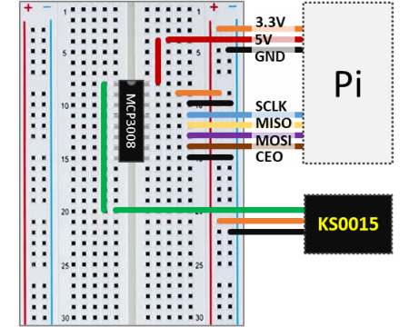
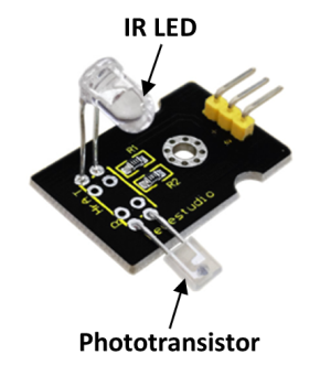
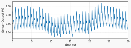
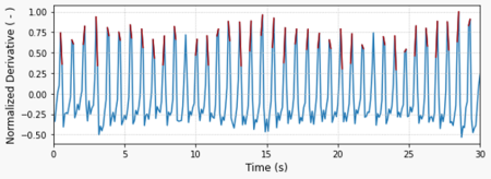
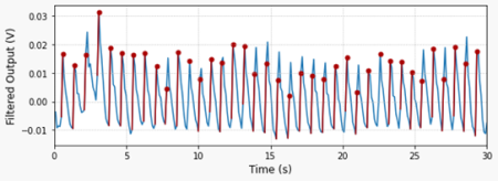
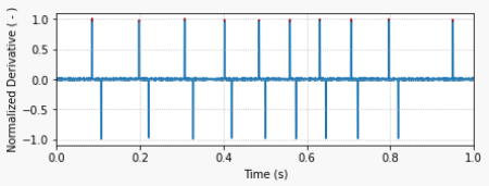
    Mean value = 6.3   |   [4, 7, 1, 11, 6, 8, 9, 3, 12, 2]

As a final remark, in the Pulse Rate Monitor post, the buffer that was used is not a true circular buffer, since the elements in the arrays are shifted by one position for every new value being sampled. Because the buffer is relatively small (200 elements) and the sampling period of the data is reasonably large (0.1s) this solution does not constitute a problem. You can check out the code that implements a true ring buffer for the monitor on my GitHub page.

Pulse Rate Monitor with Raspberry Pi

Pulse Rate Monitor with Raspberry Pi

Pulse rate can be detected using a variety of physical principles. One way of doing it is by applying infrared light to one side of the tip of your finger and sensing the “output” on the other side with a phototransistor. The blood flow through the capillaries at the finger tip fluctuates with the same frequency (rate) of your pulse. That fluctuation can be detected after processing the signal captured by the sensor.

Keyestudio has a rudimentary pulse rate monitor (KS0015) that does the trick. In this post we will go over the signal processing and how to display the pulse rate in real time. Since the KS0015 outputs an analog signal, it has to be used with the MCP3008 analog-to-digital converter chip, as illustrated in the schematics below.

As noted in previous posts, adopting a reference voltage of 3.3V for the MCP3008 provides the best resolution for the analog-to-digital conversion. The sensor output therefore has to be no greater than 3.3V, which can be achieved by using 3.3 instead of 5V as the supply voltage for the KS0015.

The very first thing to do is to look at the signal coming from the sensor as the tip of my index finger is placed between the IR LED and the phototransistor. The plot on the left can be generated by running the Python code below.

By inspecting the program, the first thing to observe is the sampling period (tsample) of 0.02 s. Since we don’t know much about the signal, it’s always good to start with a smaller value. The second thing is the wait time of 5 seconds before collecting any data. After tinkering around for a bit, I realized that the sensor is very sensitive to finger movements. Therefore, waiting for the signal to “settle down” really helps.

# Importing modules and classes
import time
import numpy as np
import matplotlib.pyplot as plt
from gpiozero import MCP3008


# Defining function for plotting
def make_fig():
    # Creating Matplotlib figure
    fig = plt.figure(
        figsize=(8, 3),
        facecolor='#f8f8f8',
        tight_layout=True)
    # Adding and configuring axes
    ax = fig.add_subplot(xlim=(0, max(t)))
    ax.set_xlabel('Time (s)', fontsize=12)
    ax.grid(linestyle=':')
    # Returning axes handle
    return ax


# Creating object for the pulse rate sensor output
vch = MCP3008(channel=0, clock_pin=11, mosi_pin=10, miso_pin=9, select_pin=8)

# Assigning some parameters
tsample = 0.02  # Sampling period for code execution (s)
tstop = 30  # Total execution time (s)
vref = 3.3  # Reference voltage for MCP3008
# Preallocating output arrays for plotting
t = []  # Time (s)
v = []  # Sensor output voltage (V)

# Waiting for 5 seconds for signal stabilization
time.sleep(5)

# Initializing variables and starting main clock
tprev = 0
tcurr = 0
tstart = time.perf_counter()
# Running execution loop
print('Running code for', tstop, 'seconds ...')
while tcurr <= tstop:
    # Getting current time (s)
    tcurr = time.perf_counter() - tstart
    # Doing I/O and computations every `tsample` seconds
    if (np.floor(tcurr/tsample) - np.floor(tprev/tsample)) == 1:
        # Getting current sensor voltage
        valuecurr = vref * vch.value
        # Assigning current values to output arrays
        t.append(tcurr)
        v.append(valuecurr)
    # Updating previous time value
    tprev = tcurr

print('Done.')
# Releasing GPIO pins
vch.close()

# Plotting results
ax = make_fig()
ax.set_ylabel('Sensor Output (V)', fontsize=12)
ax.plot(t, v, linewidth=1.5, color='#1f77b4')
ax = make_fig()
ax.set_ylabel('Sampling Period (ms)', fontsize=12)
ax.plot(t[1::], 1000*np.diff(t), linewidth=1.5, color='#1f77b4')

Digital Filtering and Pulse Detection

In this stage of the signal processing, let’s put some of the content of previous posts to good use. More specifically digital band-pass filtering and event detection for the pulse signal.

First let’s remove the low and high frequency components of the signal that are outside the band of interest. I chose 0.5 and 5 Hz (30 and 300 beats per minute) as the cutoff frequencies. That seems to be a reasonable bandwidth to account for the filter attenuation at the cutoff frequencies, as well as for the human heart “range of operation”.

Then, let’s calculate the derivative of the signal so it’s easier to detect the pulse events. By normalizing the derivative based on its maximum value, the signal amplitude becomes more consistent and therefore a single value threshold can be used. In this case 25% of the maximum value.

The plot on the top shows the normalized derivative of the filtered signal. In red are the trigger events detected by the function find_cluster, which I placed inside the module utils.py . As usual, all the code for this post can be found on my GitHub page.

The plot on the bottom shows the identified trigger events (red dots) displayed on the filtered sensor output signal.

The Python program below is an extension of the one in the previous section, where the digital filter and the trigger detection features are now incorporated. The pulse rate is calculated using the median of the time difference between two consecutive trigger events. In this case, using the median instead of the mean is recommended since it makes the calculation more robust to outliers.

Running the code will generate the two graphs shown above and print the median pulse rate for the corresponding (30-second) data acquisition window. You will notice that the signal amplitude is fairly small (approx. 30 mV) and very sensitive to the finger tip location. It might take a few tries to find the correct position and pressure for the finger.

# Importing modules and classes
import time
import numpy as np
import matplotlib.pyplot as plt
from gpiozero import MCP3008
from utils import find_cluster


# Defining function for plotting
def make_fig():
    # Creating Matplotlib figure
    fig = plt.figure(
        figsize=(8, 3),
        facecolor='#f8f8f8',
        tight_layout=True)
    # Adding and configuring axes
    ax = fig.add_subplot(xlim=(0, max(t)))
    ax.set_xlabel('Time (s)', fontsize=12)
    ax.grid(linestyle=':')
    # Returning axes handle
    return ax


# Creating object for the pulse rate sensor output
vch = MCP3008(channel=0, clock_pin=11, mosi_pin=10, miso_pin=9, select_pin=8)

# Assigning some parameters
tsample = 0.1  # Sampling period for code execution (s)
tstop = 30  # Total execution time (s)
vref = 3.3  # Reference voltage for MCP3008
# Preallocating output arrays for plotting
t = np.array([])  # Time (s)
v = np.array([])  # Sensor output voltage (V)
vfilt = np.array([])  # Filtered sensor output voltage (V)

# Waiting for 5 seconds for signal stabilization
time.sleep(5)

# First order digital band-pass filter parameters
fc = np.array([0.5, 5])  # Filter cutoff frequencies (Hz)
tau = 1/(2*np.pi*fc)  # Filter time constants (s)
# Filter difference equation coefficients
a0 = tau[0]*tau[1]+(tau[0]+tau[1])*tsample+tsample**2
a1 = -(2*tau[0]*tau[1]+(tau[0]+tau[1])*tsample)
a2 = tau[0]*tau[1]
b0 = tau[0]*tsample
b1 = -tau[0]*tsample
# Assigning normalized coefficients
a = np.array([1, a1/a0, a2/a0])
b = np.array([b0/a0, b1/a0])
# Initializing filter values
x = [vref*vch.value] * len(b)  # x[n], x[n-1]
y = [0] * len(a)  # y[n], y[n-1], y[n-2]
time.sleep(tsample)

# Initializing variables and starting main clock
tprev = 0
tcurr = 0
tstart = time.perf_counter()
# Running execution loop
print('Running code for', tstop, 'seconds ...')
while tcurr <= tstop:
    # Getting current time (s)
    tcurr = time.perf_counter() - tstart
    # Doing I/O and computations every `tsample` seconds
    if (np.floor(tcurr/tsample) - np.floor(tprev/tsample)) == 1:
        # Getting current sensor voltage
        valuecurr = vref * vch.value
        # Assigning sensor voltage output to input signal array
        x[0] = valuecurr
        # Filtering signals
        y[0] = -np.sum(a[1::]*y[1::]) + np.sum(b*x)
        # Updating output arrays
        t = np.concatenate((t, [tcurr]))
        v = np.concatenate((v, [x[0]]))
        vfilt = np.concatenate((vfilt, [y[0]]))
        # Updating previous filter output values
        for i in range(len(a)-1, 0, -1):
            y[i] = y[i-1]
        # Updating previous filter input values
        for i in range(len(b)-1, 0, -1):
            x[i] = x[i-1]
    # Updating previous time value
    tprev = tcurr

print('Done.')
# Releasing pins
vch.close()

# Calculating and normalizing sensor signal derivative
dvdt = np.gradient(vfilt, t)
dvdt = dvdt/np.max(dvdt)
# Finding heart rate trigger event times
icl, ncl = find_cluster(dvdt>0.25, 1)
ttrigger = t[icl]
# Calculating heart rate (bpm)
bpm = 60/np.median(np.diff(ttrigger))
print("Heart rate = {:0.0f} bpm".format(bpm))

# Plotting results
ax = make_fig()
ax.set_ylabel('Normalized Derivative ( - )', fontsize=12)
ax.plot(t, dvdt, linewidth=1.5, color='#1f77b4', zorder=0)
for ik, nk in zip(icl, ncl):
    if ik+nk < len(t):
        ax.plot(t[ik:ik+nk], dvdt[ik:ik+nk], color='#aa0000')
ax = make_fig()
ax.set_ylabel('Filtered Output (V)', fontsize=12)
ax.plot(t, vfilt, linewidth=1.5, color='#1f77b4', zorder=0)
for ik, nk in zip(icl, ncl):
    ax.plot(t[ik:ik+nk], vfilt[ik:ik+nk], color='#aa0000')
    ax.scatter(t[ik+1], vfilt[ik+1], s=25, c='#aa0000')

Real-time Pulse Rate Detection

Now that we have the pulse rate detection and calculation working, we can modify the code from the previous section to add the real-time display of the pulse rate. For this step, we will use a 7-segment LED display with a TM1637 chip. In case you don’t have one, all the calls for the tm object in the code below should be removed and a simple

print("Heart rate = {:0.0f} bpm".format(bpm))

can be used to replace the code line

tm.number(int(bpm))

Also, notice how we are using a circular buffer (tbuffer) of 20 seconds that holds the signal for the pulse rate calculation. The buffer is updated every tsample seconds and the actual pulse rate calculation occurs every tdisp seconds. Through comparison with the previous program, you can see how the bpm calculation is now placed inside the execution loop, hence happening in real-time.

# Importing modules and classes
import time
import numpy as np
import matplotlib.pyplot as plt
import tm1637
from gpiozero import MCP3008
from utils import find_cluster


# Defining function for plotting
def make_fig():
    # Creating Matplotlib figure
    fig = plt.figure(
        figsize=(8, 3),
        facecolor='#f8f8f8',
        tight_layout=True)
    # Adding and configuring axes
    ax = fig.add_subplot(xlim=(0, max(t)))
    ax.set_xlabel('Time (s)', fontsize=12)
    ax.grid(linestyle=':')
    # Returning axes handle
    return ax


# Creating object for the pulse rate sensor output and LED display
vch = MCP3008(channel=0, clock_pin=11, mosi_pin=10, miso_pin=9, select_pin=8)
tm = tm1637.TM1637(clk=18, dio=17)

# Assigning some parameters
tsample = 0.1  # Sampling period for code execution (s)
tstop = 60  # Total execution time (s)
tbuffer = 20  # Data buffer length(s)
tdisp = 1  # Display update period (s)
vref = 3.3  # Reference voltage for MCP3008
# Preallocating circular buffer arrays for real-time processing
t = np.array([])  # Time (s)
v = np.array([])  # Sensor output voltage (V)
vfilt = np.array([])  # Filtered sensor output voltage (V)

# Waiting for 5 seconds for signal stabilization
time.sleep(5)

# First order digital band-pass filter parameters
fc = np.array([0.5, 5])  # Filter cutoff frequencies (Hz)
tau = 1/(2*np.pi*fc)  # Filter time constants (s)
# Filter difference equation coefficients
a0 = tau[0]*tau[1]+(tau[0]+tau[1])*tsample+tsample**2
a1 = -(2*tau[0]*tau[1]+(tau[0]+tau[1])*tsample)
a2 = tau[0]*tau[1]
b0 = tau[0]*tsample
b1 = -tau[0]*tsample
# Assigning normalized coefficients
a = np.array([1, a1/a0, a2/a0])
b = np.array([b0/a0, b1/a0])
# Initializing filter values
x = [vref*vch.value] * len(b)  # x[n], x[n-1]
y = [0] * len(a)  # y[n], y[n-1], y[n-2]
time.sleep(tsample)

# Initializing variables and starting main clock
tprev = 0
tcurr = 0
tstart = time.perf_counter()
# Running execution loop
tm.show('Hold')
print('Running code for', tstop, 'seconds ...')
print('Waiting', tbuffer, 'seconds for buffer fill.')
while tcurr <= tstop:
    # Getting current time (s)
    tcurr = time.perf_counter() - tstart
    # Doing I/O and computations every `tsample` seconds
    if (np.floor(tcurr/tsample) - np.floor(tprev/tsample)) == 1:
        # Getting current sensor voltage
        valuecurr = vref * vch.value
        # Assigning sensor voltage output to input signal array
        x[0] = valuecurr
        # Filtering signals
        y[0] = -np.sum(a[1::]*y[1::]) + np.sum(b*x)
        # Updating circular buffer arrays
        if len(t) == tbuffer/tsample:
            t = t[1::]
            v = v[1::]
            vfilt = vfilt[1::]
        t = np.concatenate((t, [tcurr]))
        v = np.concatenate((v, [x[0]]))
        vfilt = np.concatenate((vfilt, [y[0]]))
        # Updating previous filter output values
        for i in range(len(a)-1, 0, -1):
            y[i] = y[i-1]
        # Updating previous filter input values
        for i in range(len(b)-1, 0, -1):
            x[i] = x[i-1]
    # Processing signal in the buffer every `tdisp` seconds
    if ((np.floor(tcurr/tdisp) - np.floor(tprev/tdisp)) == 1) & (tcurr > tbuffer):
        # Calculating and normalizing sensor signal derivative
        dvdt = np.gradient(vfilt, t)
        dvdt = dvdt/np.max(dvdt)
        # Finding heart rate trigger event times
        icl, ncl = find_cluster(dvdt>0.25, 1)
        ttrigger = t[icl]
        # Calculating and displaying pulse rate (bpm)
        bpm = 60/np.median(np.diff(ttrigger))
        tm.number(int(bpm))
    # Updating previous time value
    tprev = tcurr

print('Done.')
tm.show('Done')
# Releasing pins
vch.close()
Band-pass Filter

Band-pass Filter

A band-pass filter attenuates both low and high frequency components of a signal and therefore, as the name suggests, allows for a band of frequencies to pass through. In this post, we will briefly go over an analog implementation of this type of filter by cascading high-pass and low-pass passive analog filters. I will also go through a digital implementation using Python, as seen on the post Joystick with Raspberry Pi.

The RC circuit diagram shows the high- and low-pass filters in a cascaded arrangement. The cutoff frequency (rad/s) for the high-pass is and for the low-pass. In terms of time constants (which will be helpful later with conciseness), we have respectively and .

For example, a band-pass filter with cutoff frequencies of approximately 0.1 and 2 Hz can be realized with, , , and . Or, using time constants, and .

That’s about it for the analog implementation of a first-order band-pass filter. Let’s see how we can derive the digital version of the same filter and have it ultimately implemented in Python code (at the bottom of this post if you want to skip the technical mumbo jumbo).

Continuous Filter

The first step is to come up with a mathematical representation of the band-pass filter in the analog (continuous) domain. More specifically, as already mentioned in the PID tuning post, let’s work with the Laplace transform (or s-domain), which conveniently turns differential equations into much easier to solve polynomial equations.

In the case of the RC circuit for the band-pass filter, we want to find the transfer function between the output voltageand the input voltage. In other words, between the raw and the filtered signals.

The relationships between voltage and current for the resistor and capacitor are given by:

and

In the s-domain, the derivative operatoris “replaced” with the algebraic s operator:

and

The filter can be separated into two filters (a high-pass and a low-pass), where distinct transfer functions betweenand, as well as betweenand , can be derived and then combined.

Solving the system’s first equation (below) for the current and substituting in the second equation gives:

And rearranging as a transfer function:

Solving the system’s first equation (below) for the current and substituting in the second equation gives:

And rearranging like the high-pass case:

Finally, solving the function for the low-pass filter forand substituting the result in the function for the high-pass filter, will lead to the transfer function of the band-pass filter below (also shown in terms of time constants and descending powers of s):

Discrete Filter

The next task is to convert the continuous system to a discrete one. Similarly to the continuous domain, where the derivative operatoris represented by the operator s, the discrete domain has the operator z. (or 1) corresponds to the current time step discrete value, corresponds to the previous value , to the value before the previous one, and so on.

As seen in the post about digital filtering, for a discrete system with sampling period, the derivative of a continuous variable can be approximated by the backward difference below:

And in terms of operators, we can write:

Substituting s in the continuous transfer function for the band-pass filter gives the equation in the z-domain below. Note also that, because we are talking about a filter for any type of signal, the voltages were replaced by more general input and output variables.

Carrying out the math so we can regroup in terms of descending powers of z, and multiplying both top and bottom by, leads to:

We can then rearrange the z transfer function above to resemble a difference equation:

Where:

At last, the equation above can be brought to a more useful difference equation form, by replacing the z operators by their corresponding discrete system values:

Python Code for Band-Pass Filter

The following Python program implements the digital filter with a fictitious signal comprised of three sinusoidal waves with frequencies 0.01, 0.5, and 25 Hz. The low and high cutoff frequencies of the filter are 0.1 and 2 Hz, therefore allowing only the 0.5 Hz component of the original signal to pass through.

By analyzing the code, it is straightforward to identify the filter coefficients determined in the previous section. The difference equation was implemented in the more general form

where the sets of coefficientsandare normalized by the coefficientof the output. This approach allows for any type of digital filter to be used in the code, as long as the normalized coefficients are defined.

# Importing modules and classes
import numpy as np
from utils import plot_line

# "Continuous" signal parameters
tstop = 20  # Signal duration (s)
Ts0 = 0.0002  # Time step (s)
fs0 = 1/Ts0  # Sampling frequency (Hz)
# Discrete signal parameters
tsample = 0.01  # Sampling period for code execution (s)
# Preallocating output arrays for plotting
tn = []
xn = []
yn = []

# Creating arbitrary signal with multiple sine functions
freq = [0.01, 0.5, 25]  # Sine frequencies (Hz)
ampl = [0.4, 1.0, 0.2]  # Sine amplitudes
t = np.arange(0, tstop+Ts0, Ts0)
xs = np.zeros(len(t))
for ai, fi in zip(ampl, freq):
    xs = xs + ai*np.sin(2*np.pi*fi*t)

# First order digital band-pass filter parameters
fc = np.array([0.1, 2])  # Band-pass cutoff frequencies (Hz)
tau = 1/(2*np.pi*fc)  # Filter time constants (s)
# Filter difference equation coefficients
a0 = tau[0]*tau[1]+(tau[0]+tau[1])*tsample+tsample**2
a1 = -(2*tau[0]*tau[1]+(tau[0]+tau[1])*tsample)
a2 = tau[0]*tau[1]
b0 = tau[0]*tsample
b1 = -tau[0]*tsample
# Defining normalized coefficients
a = np.array([1, a1/a0, a2/a0])
b = np.array([b0/a0, b1/a0])
# Initializing filter values
x = np.array([0.0]*(len(b)))  # x[n], x[n-1], x[n-2], ...
y = np.array([0.0]*(len(a)))  # y[n], y[n-1], y[n-2], ...

# Executing DAQ loop
tprev = 0
tcurr = 0
while tcurr <= tstop:
    # Doing I/O computations every `tsample` seconds
    if (np.floor(tcurr/tsample) - np.floor(tprev/tsample)) == 1:
        # Simulating DAQ device signal acquisition
        x[0] = xs[int(tcurr/Ts0)]
        # Filtering signal
        y[0] = -np.sum(a[1::]*y[1::]) + np.sum(b*x)
        # Updating previous input values
        for i in range(len(b)-1, 0, -1):
                x[i] = x[i-1]
        # Updating previous output values
        for i in range(len(a)-1, 0, -1):
                y[i] = y[i-1]
    # Updating output arrays
    tn.append(tcurr)
    xn.append(x[0])
    yn.append(y[0])
    # Incrementing time step
    tprev = tcurr
    tcurr += Ts0

# Plotting results
plot_line(
    [t, tn], [xs, yn], yname=['X Input', 'Y Output'],
    legend=['Raw', 'Filtered'], figsize=(1300, 250)
)

The plot below shows the code output where the low frequency drift and the high frequency noise are almost fully removed from the signal, while the desired component of 0.5 Hz is preserved.

Event Detection in Signal Processing

Event Detection in Signal Processing

One thing I always come across when analyzing time-based data is the need to identify events such as changes in signal level, triggers, among others. Many years ago I created a MATLAB function that can find clusters of data values inside a time series. It returns the indexes of the starting point of each cluster, with the corresponding number of samples within each cluster. I have been using the Python version of the function quite a bit recently. Apparently it never gets old!

By doing the proper manipulation of the data, virtually any type of event can be detected and extracted from the time series.

The example on the left shows a generic signal where we search for clusters of data (or events) with values greater than zero. In most cases, it’s good practice to apply a post-processing filter to the signal as the very first step of the data analysis.

The code for the python function used to find the clusters is shown below. Let’s get started by showing some basic usage and then some more interesting cases.

def find_cluster(x, xval):
    """
    Find clusters of data in an ndarray that satisfy a certain condition.


    :param x: The array containing the data for the cluster search.
    :type x: ndarray

    :param xval: The value of x that has to be satisfied for clustering.
    :type xval: integer, float


    :returns: 2-tuple

        * i0:
            The index of each cluster starting point.

        * clustersize:
            The corresponding lengths of each cluster.

    :rtype: (list, list)


    Example
    -------
        >>> x = np.int32(np.round(np.random.rand(20)+0.1))
        >>> i0, clustersize = find_cluster(x, 1)

    """
    # Cluster information list
    a = []
    # Initial (place holder) values for cluster start and end points
    kstart = -1
    kend = -1
    # Going through each value of x
    for i, xi in enumerate(x):
        if xi == xval:
            # Assigning cluster starting point
            if kstart == -1:
                kstart = i
            # Assigning cluster end point for particular case
            # when there is an xval in the last position of x
            if i == len(x)-1:
                kend = i
        else:
            # Assigning cluster end point
            if kstart != -1 and kend == -1:
                kend = i-1
        # Updating cluster information list
        # and resetting kstart and kend
        if kstart != -1 and kend != -1:
            a.append(kstart)
            a.append(kend)
            kstart = -1
            kend = -1
    # Assigning indeces of cluster starting points
    # (Every other list element starting from position 0)
    i0 = a[0:-1:2]
    # Assigning cluster sizes
    # (Every other list element starting from position 1)
    clustersize = list(np.array(a[1::2]) - np.array(i0) + 1)
    # Case where cluster size is ZERO
    if len(i0) == 0:
        i0 = []
        clustersize = []
    return i0, clustersize

The example in the doc string above generates a random array x of zeros and ones, in which we use the function to find the clusters of values equal to 1. By running it, one should get something like the results shown below. i0 contains the starting indexes of the clusters of 1s and clustersize contains the number of elements in each cluster.

>>> x = np.int32(np.round(np.random.rand(20)+0.1))
>>> i0, clustersize = find_cluster(x, 1)

>>> x
array([1, 1, 1, 0, 1, 0, 1, 1, 1, 1, 1, 1, 0, 1, 1, 0, 0, 1, 1, 0])

>>> i0
[0, 4, 6, 13, 17]

>>> clustersize
[3, 1, 6, 2, 2]

Finding Signal Peaks

Let’s use the signal from the top of the post and find the signal peaks above 1 and below -1, as illustrated on the left.

The code snippet used to find the peaks as well as the peak values can be seen below. The complete code for it and for all the examples in this post can be found here.

# Finding positive peaks greater than 1
imax = []
icl, ncl = find_cluster(x>1, 1)
for ik, nk in zip(icl, ncl):
    imax.append(ik+np.argmax(x[ik:ik+nk])-1)
# Finding negative peaks smaller than 1
imin = []
icl, ncl = find_cluster(x<-1, 1)
for ik, nk in zip(icl, ncl):
    imin.append(ik+np.argmin(x[ik:ik+nk])-1)
>>> np.round(x[imax], 2)
array([1.3 , 1.03, 1.47, 1.06, 1.18, 1.53, 1.21, 1.19])

>>> np.round(x[imin], 2)
array([-1.25, -1.19, -1.53, -1.24, -1.07, -1.47, -1.08, -1.3 ])

Finding Trigger Edges

find_cluster can be very useful for determining trigger events in a recorded time series. Unlike most other signals, I usually do not filter a trigger signal, since having a sharp rising edge (at the expense of noise) is critical for a more exact event determination.

The derivative of the trigger signal is then used to determine the rising edges, as shown in the second plot on the left. A threshold value of 0.5 for the derivative (normalized by its maximum value) can be used to locate the trigger edges.

The code snippet below shows how to do it for a fictitious recorded data set.

# Calculating and normalizing trigger signal derivative
dxdt = np.gradient(x, t)
dxdt = dxdt/np.max(dxdt)

# Finding trigger event times using derivative theshold
icl, ncl = find_cluster(dxdt>0.5, 1)
ttrigger = t[icl]
>>> ttrigger
array([0.0845, 0.1975, 0.3065, 0.402 , 0.485 , 0.559 , 0.6305, 0.7055, 0.796 , 0.9495])
Python DAC Class

Python DAC Class

Creating a class to represent a Raspberry Pi digital-to-analog converter is a good example on how to put together the concepts we have been exploring in some of the previous posts. More specifically, DAC with Raspberry Pi and Classes vs. Functions in Python. Besides a Raspberry Pi and a couple of resistors and capacitors, we need an additional DAQ device to calibrate our Pi DAC output.

In the post DAC with Raspberry Pi, we used an MCP3008 to measure (and calibrate) the DAC output. This time around I will follow my recommendation of not using the same DAQ to generate and measure the output, using instead a LabJack U3. While a LabJack is not a calibration DAQ device, it is far more accurate than a Pi, therefore moving us in the right direction when it comes to choosing a calibration device.

The setup is quite simple: On the Pi side, a GPIO pin used as PWM input to the the low-pass filter and a GND pin. On the U3 side, the RC filter output (which is our DAC output) is connected to the analog input port AIN0, while the GND port is connected to the same GND as the Pi.

The U3 is connected to a separate computer via USB and will be running a variation of the code that can be found on my GitHub page. The Python package that I made containing the LabJack U3 class can be installed from the PyPI (Python Package Index) page.

As before, the cascaded second order filter is made of two first order low-pass RC filters, where R = 1 kΩ and C = 10 μF.

Of course, if you don’t have a LabJack, a digital multimeter should do the trick and allow you to measure the DAC output in order to do its calibration. I chose to use a LabJack to gain some insight on the DAC output signal by using its 50 kHz streaming capability (and because an oscilloscope is not among my few possessions).

The next step is to layout what our DAC class should look like. You may want to put down a “skeleton” of the class, as shown below, with a brief description of what the attributes are and what the methods do. Using the reserved word pass allows for placeholders for the methods to be easily created and filled out later.

class DAC:

    def __init__(self):
        # Class constructor
        self._vref = 3.3  # Reference voltage output
        self._slope = 1  # Output transfer function slope
        self._offset = 0  # Output transfer function intercept

    def __del__(self):
        # Class destructor
        # - makes sure GPIO pins are released
        pass

    def reset_calibration(self):
        # Resets the DAC slope and offset values
        pass

    def set_calibratio(self):
        # Sets the DAC slope and offset with calibration data
        pass

    def get_calibration(self):
        # Retrieves current slope and offset values
        pass

    def set_output(self):
        # Sets the DAC output voltage to the desired value
        pass

One of the nice things about using classes is that it’s easy to add (or remove) attributes and methods as you code away. And even better, if you’re using the interactive session of VS Code, saved updates to your methods are immediately reflected in any instance of the class that is present in the session’s “workspace” (to use a MATLAB term, for those familiar with it). In other words, if you were to call that method again using dot notation, it would behave based on the latest modifications that you saved.

In the case of our example, the attributes need to hold the values of a reference voltage (Pi’s 3.3 V if you’re not using any OpAmp with your filter) and the calibration parameters which are used so the DAC can output the correct set voltage value.

from gpiozero import PWMOutputDevice


class DAC:

    def __init__(self, dacpin=12):

        # Checking for valid hardware PWM pins
        if dacpin not in [12, 13, 18, 19]:
            raise Exception('Valid GPIO pin is: 12, 13, 18, or 19')
        # Assigning attributes
        self._vref = 3.3  # Reference voltage output
        self._slope = 1  # Output transfer function slope
        self._offset = 0  # Output transfer function intercept
        # Creating PWM pin object
        self._dac = PWMOutputDevice(dacpin, frequency=700)

    def __del__(self):

        # Releasing GPIO pin
        self._dac.close()

    def reset_calibration(self):
        self._slope = 1
        self._offset = 0

    def set_calibration(self, slope, offset):
        self._slope = slope
        self._offset = offset

    def get_calibration(self):
        print('Slope = {:0.4f} , Offset = {:0.4f}'.format(
            self._slope, self._offset))

    def set_output(self, value):

        # Limiting output
        output = self._slope*value/self._vref + self._offset
        if output > 1:
            output = 1
        if output < 0:
            output = 0
        # Applying output to GPIO pin
        self._dac.value = output

As far as the methods are concerned, a constructor and a destructor, being the latter a good idea so the GPIO pin can be released once you’re done using the class instance. Also, a group of methods to deal with the DAC calibration and a single method to set the DAC output value. Notice that the attribute names start with an underscore. That’s a loose Python convention to define private properties (or methods, if I were to use the underscore as the first character of the method name), unlike other programming languages which are more rigorous about it by making you explicitly define what’s private. The general idea of private properties (or methods) is that they’re not supposed to be accessible directly by the user of the program, therefore, being accessed internally by the code.

DAC Calibration

First, we create an instance of the DAC class on GPIO pin 18: mydac = DAC(dacpin=18)

Then, the output calibration is done with two output settings (0.5 and 3.0 V) using the method: mydac.set_output(0.5) and mydac.set_output(3.0). Each time the output is read using the streaming feature of the LabJack U3, as shown on the left. The high frequency noise in the signal is quite apparent and is a most likely due to the limitations of the Raspberry Pi hardware. For the two desired outputs of 0.5 and 3.0 V, the corresponding mean actual values are 0.614 and 2.854 V. Because the system response is linear, two data points are sufficient.

The slope and offset are calculated as slope = (3.0 – 0.5) / (2.854 – 0.614) = 1.116, and offset = 0.5 – (3.0 – 0.5) / (2.854 – 0.614) x 0.614 = -0.185. The calibrated values are applied to the DAC instance using the method mydac.set_calibration(1.116, -0.185). If a new calibration has to be done, the default values of 1 and 0 can be restored by using the method mydac.reset_calibration(). As mentioned earlier, the private attributes _slope and _offset are not dealt with directly by the user but instead through different methods. Of course, in this simple example, they could be changed directly by doing mydac._slope = 1.116 and mydac._offset = -0.185. In more complex situations there might be a few good reasons to avoid direct access to an instance’s attributes.

With the calibrated DAC, the new outputs to the same settings as before (0.5 and 3.0 V) give the results on the left, where the actual mean values are 0.493 and 3.006 V, respectively.

DAC Test

Let’s put the DAC device to the test! The Python code below can be used to generate a random sequence of steps every 0.5 seconds between 0 and 3 V (every 0.5 V). The data is collected using the LabJack U3 streaming feature and plotted in the next figure. Not too bad for our poor man’s DAC.

import time
import numpy as np
from gpiozero_extended import DAC

# Assigning parameter values
tstep = 0.5  # Interval between step changes (s)
tstop = 10  # Total execution time (s)

# Creating DAC object on GPIO pin 18
mydac = DAC(dacpin=18)
mydac.set_calibration(1.116, -0.185)

# Initializing timers and starting main clock
tprev = 0
tcurr = 0
tstart = time.perf_counter()

# Running execution loop
print('Running code for', tstop, 'seconds ...')
while tcurr <= tstop:
    # Updating analog output every `tstep` seconds with
    # random voltages between 0 and 3 V every 0.5 V
    if (np.floor(tcurr/tstep) - np.floor(tprev/tstep)) == 1:
        mydac.set_output(np.round(6*np.random.rand())/2)
    # Updating previous time and getting new current time (s)
    tprev = tcurr
    tcurr = time.perf_counter() - tstart

print('Done.')
# Releasing pin
del mydac
Digital-to-Analog Conversion

Digital-to-Analog Conversion

As the counterpart of analog-to-digital conversion, DAC will take a digital signal and convert it to an analog one. Paraphrasing what I mentioned in previous posts, ADC and DAC walk hand-in-hand bridging the gap between the continuous and discrete domains that modern machines and devices have to deal with.

Even though there are several types of DACs, I will talk about the PWM-based one, where a reference input voltage is switched (in the form of a digital train of pulses) into a low-pass analog filter, producing an analog output. Before we get there, let’s first talk about Pulse Width Modulation, a very clever way to go from the discrete to the continuous domain, invented in the mid-seventies. A PWM signal has two main characteristics: its frequency and its duty cycle.

The figure illustrates the frequency and the concept of duty cycle for a 10 Hz PWM signal. In this case, the period of the PWM is 1/fPWM = 0.1 s. The chosen duty cycle is 25 %, which corresponds to the time the output is “on” (0.025 s). During the remainder of the duration of the PWM period (0.075 s) the output is “off”. As a matter of fact, it’s the modulation of the duty cycle that will control the output level of the DAC system.

Since it’s either fully “on” or fully “off”, the PWM signal is fundamentally a digital one. It’s the frequency and duty cycle of that “on-off” train of pulses, coupled with the response of the sub-system it’s interacting with, that will result in an analog behavior of the output of the overall system, in our case the digital-to-analog converter.

As a side note, the Python code used to generate the graphs in this post can be found on my GitHub page. Make sure to check it out and experiment with the DAC parameters.

The simplest DAC implementation is shown on the left. It consists of a low-pass first-order passive RC filter connected to the PWM output signal Vref. Typically, for a TTL circuit, the voltage can be either 0 (low) or 3.3V (high).

The cutoff frequency (rad/s) of the filter is fc = 1/(RC). Along with the PWM frequency, it can be used to obtain the desired behavior of this simple DAC.

Output Ripple

The PWM signal can be thought as a sequence of low-to-high and high-to-low step inputs into the RC filter. Even with a constantly switching input, this first order system will eventually produce a near constant output. The figures below show the effect of the RC filter cutoff frequency fc as well as the PWM frequency fPWM on the amplitude of the output ripple.

As it can be observed in the plots above, the output voltage will converge to (duty cycle) x Vref , which for the duty cycle of 25 % (used in the example) produces an output of 0.825 V when Vref = 3.3 V. Also, reducing the filter cutoff frequency or increasing the PWM frequency are both effective in reducing the output signal ripple. While having a slow RC filter can greatly reduce the ripple, that will negatively affect the DAC response time when it’s subject to a change in the desired output value.

DAC Step Response

In the case of our DAC, its response time is essentially the response time of the RC filter, i.e. 1/fc = RC (with fc in rad/s). Leaving the details for a future post on analog and digital filtering, for the first order system under consideration, the response time can be defined as the time it takes for the output to reach about 63 % of its final (steady-state) value, after a step input is applied.

The next figure shows how an appropriate combination of a higher PWM frequency and a higher filter cutoff frequency can produce a faster response time, while maintaining roughly the same amplitude of the DAC output ripple. For our example, the response time based on the RC value goes from 0.16 s down to 0.04 s.

Cascaded Filters

The output ripple can be further improved by cascading two first-order RC filters, as shown below. The newly formed second-order filter will have twice the attenuation (dB/decade) above the cutoff frequency. It’s an easy-to-do improvement which is often adopted.

Practical Considerations

Just like its ADC counterpart, DACs also have an inherent quantization in the signal. The digital PWM, generated from the microprocessor clock, has a finite resolution (duty cycle levels) given by the number of bits of the PWM. Typical resolutions range from 8 to 12 bits.

Actual PWM frequencies for DAC devices are much higher than the ones used in the examples above, which were chosen mainly to illustrate the concepts. For applications involving testing of physical systems or automation, frequencies between 500 and 2000 Hz are reasonable. In audio applications, several times the highest frequency of the audible range (20 kHz) seems to be the case. That is, 100 to 200 kHz. However, just as we observed when using higher order filtering, there’s wiggle room to reduce these numbers while still having a good compromise between response time and ripple.

It’s important to make a distinction at this point: if the PWM is used to drive a DC motor directly (or with some power amplification), the motor itself will behave approximately as a first order system. Hence, there’s no need for the RC filter. In this type of application, PWM frequencies of 100 to 200 Hz are just fine.

Amplification of the DAC output beyond the typical 3.3V Vref, can be achieved by using an Op Amp (Operational Amplifier). For a simple non-inverting amplifier, the output voltage is given by:

V2 = V1(1+R1/R2)

By choosing R1 = R2 = 10 kOhm, we can double the output to accommodate a more typical 0 to 5V requirement.

In my next post, we will explore the implementation of a DAC using a Raspberry Pi and a few resistors and capacitors. The Pi has hardware enabled PWM on two of its GPIO pins, which can reach frequencies in the kHz range! That should be an interesting project.

Analog-to-Digital Conversion

Analog-to-Digital Conversion

Also known as ADC, is the process of converting a physical quantity, usually represented by a voltage at this point, to a set of bits that’s more suitable for a computer to digest. Bearing in mind that the world we live in is analog in nature and the computers we use to interact with it are digital, going from the continuous domain to the discrete domain is an integral part of most machines and devices out there.

Back in the day, when micro-processors and computers weren’t around or were still in their infancy, many systems would function entirely in the analog domain. Take for instance an old record player. From the needle running in the record tracks (a continuous profile of peaks and valleys) to the sound coming out of the speakers, the entire sequence of changes in physical quantities occurred in the analog domain. Nowadays, still on the same example, music is stored as digital content and only converted back to an analog signal when it’s time to make it to the speakers, so we can listen to it with our good old analog ears. This last process of going back from the discrete to the analog domain is handled through a digital-to-analog conversion (DAC) and will be a topic of another post. The entire process can be illustrated with the diagram below.

As I alluded to at the very top, a sensor (or more specifically a transducer) will convert the measured physical quantity to an electrical signal, and ultimately a voltage. The next step in the process is the signal conditioning where some sort of filtering will be applied to the measured voltage. Not only to avoid aliasing, which we will discuss later on, but some times to accomplish other goals, like for example remove a DC component or a very slow drift in the signal.

The next block is the analog-to-digital conversion (ADC), which has mainly two tasks to it: sampling and quantization. Once they are performed, the continuous signal will be broken down into packets of bits that the computer can now handle. We will see that the signal is not only discrete in time but also each sample can only have a finite number of values.

At the bottom half of the diagram is the flip side of the coin: the digital-to-analog (DAC) conversion, an eventual power amplification and, generally speaking, the electro-mechanical actuators.

You should also note that if we are talking about data acquisition only, the focus is the top half of the diagram. If automation is the case, then the entire diagram is in scope.

Sampling

A physical system changes its states continuously over time and it would be impractical to collect continuous data to be used by an inherently discrete system such as the computer. Using the music example, and going back several decades, data would be collected and recorded on magnetic tapes so it could be later edited, mixed, and reproduced. With the computer entering the landscape, those analog systems had their days numbered.

The sampling process occurs in an integrated circuit (IC), where an electronic switch will bring a sample of the signal into the AD converter at a fixed sampling period.

The figure on the right shows 2 seconds of an arbitrary continuous signal sampled at 0.1 seconds (or 10 Hz). The first thing to notice is that we can now store 20 data points instead of an impractical infinite number of continuous points.

There are other considerations that dictate the sampling period (or frequency) than just the amount of data that can be manipulated. The main one is the frequency content of the signal. In other words, how “fast” does the signal change over time. For good signal reconstruction in the time domain, a sampling rate of 10 to 20 times the frequency content of the signal should be used. Most importantly, it must never be below 2 times the highest frequency component of the measured signal. Otherwise, aliasing will potentially occur to the sampled data.

As a quick note, all the plots used in this post were generated using Python and the Matplotlib package. You can get the code on my GitHub page.

Nyquist Theorem and Aliasing

According to the Nyquist sampling theorem, the sampling rate should be at least two times the maximum frequency component of the measured signal. The figure below shows a 20 Hz sinusoidal signal sampled at 21 Hz. Any sampling rate below 40 Hz will result in an alias of the original signal. In this case a new 1 Hz sinusoidal wave will show up.

The frequency of the aliased signals (yes, there’s more than one alias) is not exactly intuitive, as it appears to be in the previous figure. The same original 20 Hz signal sampled at 7 Hz would also produce a 1 Hz aliased signal! Check out the Python code on my GitHub page for a couple of formulas and to explore different sampling rates.

In practical terms, it is hard to guarantee that the signal being sampled won’t contain stray frequencies above the Nyquist frequency. The best way to avoid aliasing is to use an analog low-pass filter before the signal is sampled. Even a simple passive RC filter should suffice, provided a reasonable frequency transition band to accommodate for the poor filter attenuation right above its cut-off frequency.

Back to the music example, audio is usually sampled at 44.1 kHz. Since the human ear can respond to frequencies up to about 20 kHz, sound should be sampled at least at 40 kHz. 44.1 kHz gives a Nyquist frequency of 22.05 kHz and therefore a transition band of 2.05 kHz for a filter with a cut-off frequency of 20 kHz. However, it’s not uncommon to record audio at 48 kHz (or even 96 kHz). The former gives a Nyquist frequency of 24 kHz and therefore a wider 4 kHz transition band for a low-pass filter to attenuate the signal above it’s cut-off frequency of 20 kHz.

For the classically inclined, how does 48 kHz compare with the frequency contents of the music that’s being recorded? A soprano can hit C6 (1046.5 Hz), a violin A7 (3520 Hz), and a piano C8 (4186.01 Hz). Those frequencies are well bellow the Nyquist frequency of 24 kHz and even 10 times (or more) lower than the 48 kHz sampling frequency, allowing also for good signal reconstruction in the time domain.

Quantization

The second task in the AD processing is the quantization of the sampled values. Even though your computer can deal with floating numbers (they’re still a bunch of bits in disguise), the ADC device still ships out a packet of bits for every analog sample. The analog value will be discretized based on a reference voltage and the number of bits used for the quantization.

The ideal transfer function (TF) between the analog input voltage and the digital output code is a straight line where for every possible input there’s a unique output. In other words, the ideal ADC has an infinite resolution. Because the output of the conversion is a digital value, the transfer function of a perfect ADC is in fact a staircase function where each step is 1 LSB (Least Significant Bit).

As shown in the figure, let’s consider the case with a reference voltage VREF = 2 V and a resolution of 3 bits. The step size (1 LSB) is 0.25 V, or in the general case VREF / 2n, where n is the number of bits of the ADC.

Any analog input within a step will be coded to the same digital output. For example, 0.625 to 0.875 V will be coded as 011 (or 3 in decimal representation). Using the reference voltage of 2 V, that would give us 3VREF / 8 = 0.75 V. Therefore, the quantization error goes from +0.125 V to -0.125 V. In other words +/- 0.5 LSB. This would be the case for the perfect ADC shown in the figure, more specifically a single-ended mode configuration with adjusted quantization. A good source explaining other configurations and also sources of errors that occur on an actual ADC can be found here. The full scale (FS in the figure) is VREF – 1LSB, which in the case of this example would be 1.75 V.

If a 4-bit converter is used, the quantization error for the same reference voltage drops to +/- 0.0625 V (still +/- 0.5 LSB) and the FS goes up to 1.875 V.

As we move up in bit resolution, the ADC output starts to approximate the ideal transfer function. In the case of a 10-bit ADC, the quantization error becomes +/- 0.5VREF/1024. Which in our case is approximately +/- 0.001 V, and in the general case +/- 0.05 % of the reference voltage. For a high accuracy 16-bit ADC, the error is approx. +/- 0.0008 % of the reference voltage.

Note that there are additional errors introduced in the quantization process due to offsets, non-linearities, and just noise in general in the electronic circuitry. A 12-bit converter will typically have +/- 0.13 % (instead of +/- 0.012 %) and a 16-bit a typical +/- 0.01%.

Practical Considerations

So, how high should you go with the sampling rate and number of quantization bits? How about the anti-aliasing filter? Keep in mind that faster, higher-resolution hardware comes with a steeper cost. And high sampling rates bring the burden of extra storage space and processing power.

If you are working with audio, definitely 48 kHz and 16-bit ADC for sound recording. 96 kHz (or even 172 kHz) and 24-bit if you’re a pro. And most definitely an anti-alias filter. By the way, the fact that 96 kHz is two times the 48 kHz base rate makes it very easy to down sample a recording for later reproduction: just throw away every other data point.

If you’re toying around with a Raspberry Pi, the sampling rate is the one that suits your needs. For slow changing temperatures 1 Hz is plenty. Pressures maybe 10 to 20 Hz. A 10-bit ADC MCP3008 chip is inexpensive and has plenty of resolution. An anti-aliasing filter is probably overkill. The higher frequency content of noise is also usually low amplitude and therefore shouldn’t affect you signal very much. However, it’s always a good idea to sample your data first at a higher frequency and inspect it as a function of time. Also, be careful with some typical electrical noise like the 60 Hz one caused by the AC outlet.

In a lab or instrumentation setting, 12 to 16-bit and an anti-aliasing filter, such as a simple passive RC one, should be considered. Again, try different sampling rates and filters. As I mentioned before, it’s always important to look at your data as a function of time first with as high as a sampling rate that can be run with the DAQ device at hand. Once you understand what the signal is all about, then a more conscious decision about the hardware requirements can be made.

Finally, just to have some fun with Python, below is the arbitrary signal of this post with two different sampling rates and resolutions. Observe the effects of both the sampling and the quantization on the original signal.

Fuel Flow Measurement (an automation example)

Fuel Flow Measurement (an automation example)

Some of the older engine durability test cells at Navistar needed their fuel consumption measurement system updated. The existing one was built on a dedicated IC board and finding replacement components was becoming increasingly difficult. More importantly, a newer system that was capable of interfacing with other test cell software was also a necessity.

When it comes to automating a measurement system, in addition to the automation of the measurement process itself, two other important tasks have to be kept in mind and automated as well, if possible: the task of checking if the measurement accuracy is within a given specification, and the task of calibrating the system if it is out of spec. These three automation components (the process itself, accuracy checks, and calibration) can be applied to a large group of measurement systems and industrial processes. The fuel flow measurement system belongs to this group.

With that in mind, the fuel flow measurement system consists of two physical parts: a fuel column located in the test cell and a calibration cart. The former performs the measurement task, while the latter the check and calibration tasks. If we remember the post DAQ, SBC, etc., in this particular case, a computer and a DAQ device were used to automate the system. The computer was a very capable test cell PC, that was in charge of controlling many of test cell sub-systems, being the fuel flow measurement system one of them. A single DAQ device (LabJack U6) was part of the test cell hardware and interfaced with the sensors and actuators of both the fuel column and the calibration cart. Below are the main requirements of the automation system:

  • Real-time 10 Hz monitoring of fuel flow (or consumption by the engine)
  • Automatic fuel column refill
  • Capability of manual measurements taken by the operator
  • Capability of measurements commanded by other software via UDP/IP
  • Automated fuel column calibration (fuel mass as a function of voltage)
  • Automated fuel column periodic flow accuracy check
  • Automatic report generation for calibrations and flow checks

Fuel Column

As the engine draws fuel from the column, the output current of the pressure transducer (measured as a voltage over a resistor) is processed by the automation software and a real-time fuel flow value is displayed in the graphical user interface. When the fuel level drops below a certain voltage threshold, the software operates the refill solenoid, topping off the column. This process repeats itself automatically so there’s always fuel in the column.

When a measurement is triggered, either manually or through an external software request, the fuel column is topped off first and then the fuel flow is measured and averaged for a user-defined time duration. The final value is displayed on the interface and sent to the software that made the request, if that’s the case.

An analog input port on the LabJack U6 acquires the voltage signal from the pressure transducer after it’s filtered with an anti-aliasing low-pass filter. The 110 V refill solenoid is switched on or off via a solid-state relay connected to one of the LabJack’s analog output ports.

Calibration Cart

The cart is used to characterize the relationship between the fuel mass in the column and the voltage output from the pressure transducer located at its bottom. When the column is connected to the fuel cart for a calibration procedure, a fuel pump on the cart draws fuel from the column into a container sitting on a high precision scale inside the cart. The automation software executes this procedure automatically by drawing incremental amounts of fuel. At each increment, the fuel mass value is measured by the scale. A function is then fitted to the collected data points of mass vs. voltage.

When the cart is being used to check an existing calibration, the flow measured by the automation software is compared to the fuel flow calculated by using the actual mass collected inside the container on top of the high precision scale, over a certain amount of time.

An analog output port on the LabJack U6 is used to turn the cart pump on or off through a solid-state relay. Communication between the automation software and the fuel scale is done using a RS-232 serial cable connected directly to the test cell PC where the software is installed.

Reporting

Fuel column calibration report example
Fuel column flow check report example

Keeping track of calibrations and flow checks is critical for the engine lab compliance with quality norms and, generally speaking, is an important part of an automated system. To that end, Excel-based reports are automatically generated for each calibration procedure or flow check. These are stored in a database and can be later retrieved and analyzed.

Fuel Column Simulator

Finally, because engine test cells are running most of the time, it was difficult to find a window of opportunity to develop the automation software that controls the fuel column.

To work around this limitation, a fuel column simulator that also includes the calibration cart functionality was created.

Fuel column simulator GUI

The filling and emptying behavior of the column, as well as the other automation system components, was closely matched in the simulator. The main ones were:

  • refill solenoid valve on/off
  • calibration cart pump on/off
  • fuel scale serial communication
  • fuel scale tare operation

Summary

The main idea of this post was to show a real application of the concepts of data acquisition and automation using a computer and a DAQ device. All the elements presented here can be applied to a wide variety of systems. While this one wasn’t too complex, it was part of a larger project to fully automate an engine test cell. Nonetheless, even more complex automation projects can usually be broken down into smaller, more manageable pieces. And that’s how you go about it.

Back to top

DAQ, SBC, etc.

DAQ, SBC, etc.

DAQs, SBCs, Embedded Systems, and computers. How do they all fit together? Let’s first spell out the acronyms: DAQ stands (surprisingly) for Data Acquisition in general. It includes the software and hardware side of things. For this discussion, let’s stick to the hardware side. SBC stands for Single Board Computer. Something like your PC, but where everything that’s inside the box is on one single integrated circuit board. Furthermore, the SBCs we are interested in also have GPIO (General Purpose Input and Output), which we’ll get to later.

When we talk about data acquisition (in the broader sense) and automation, we are looking to interface the real world with a digital system, through sensors and actuators. Information will be collected or sensed from the real world, some sort of analysis or decisions will be made, and if we are doing automation, an action will be taken back into the real world.

As illustrated below, there are mostly three ways to put all the pieces together. Starting from the left, the most flexible, and usually most expensive arrangement, is a computer running on top of a DAQ device. In this type of application, it’s important to be able reconfigure your system to whatever your data acquisition needs are. A lab is usually where you will find this type of system, where the accuracy of what you’re measuring also plays a big role. A short list of DAQ devices should include LabJack, National Instruments and Yokogawa.

In the middle are the SBCs. Usually far less powerful than your computer, but still a fully functional computer. The SBCs of interest to us are the ones that also have GPIO pins. These General Purpose Input and Output pins enable a connection between the sensors/actuators and the software in the computer interacting with them. They are very cost-friendly and are used in education or in DIY projects, where accuracy and reliability are less critical. Also, the SBCs will mostly handle only digital signals. Any conversion from the real world analog signal to something the SBC can understand has to happen in the sensor or a separate ADC (Analog-to-Digital Conversion) component. Most DAQs, on the other hand, have the capability to handle both digital and analog signals, doing the needed conversions and providing the computer with a signal it can understand. A popular example of an SBC is the Raspberry Pi.

On the right hand side of the figure are the embedded systems, which by the way, are all around us. From the very sophisticated automotive ones (engine control units, transmission controllers, etc.) to the less glamorous ones, like the one in your dishwasher, these are dedicated computers, or more specifically micro-processors that only do one group of tasks and are designed to work with a specific set of sensors and actuators. They are more cost effective due to mass production and some of them are extremely fast, performing real-time calculations so all the actuation decisions can be made on-the-go. Depending on the application, reliability is quite critical. You don’t want the micro-processors in that air plane having to be rebooted amid flight. A good example of a very affordable embedded system is the Arduino.

A note on speed

When it comes to collecting data, it’s not uncommon to have an execution loop in the code that controls the acquisition. That is especially the case with automation. The tasks within an execution loop can be primarily grouped into either computations or I/O. The first group contains all activities where some processing of the data is done. The second group is where the inputs from and outputs to the real world are occurring, through a DAQ device or built-in I/O.

How fast an execution loop can run depends on how fast the tasks within each of those two groups can run. To some extent, it will come down to the hardware that’s being used for either the computation or the I/O. Let’s not forget that the number of data channels that are being handled is also an important factor. The better (and usually more expensive) the hardware, the faster it can run. Generally speaking, a computer with a DAQ device should have no problem with the computation part but may be held back by the DAQ device I/O.

On the other end of the spectrum, an embedded system, due to cost constraints, doesn’t have the computing power of a regular PC and may face some limits on how many computations can be performed. That is an important aspect, especially because these types of systems are used in real-time applications. The time it takes to get the sensor input data, do computations, and set the output actuator data (for one execution step) has to fit within the time frame of what’s happening with the real world that the embedded system is interacting with.

In terms of numbers (depending on complexity of calculations, hardware, sensors, and number of channels), a computer with a DAQ device should be able to run execution loops in the 10 to 100 Hz range. SBCs, which have the built-in I/O, can bring that number to 200 Hz or more. Embedded systems are all over the execution frequency range. Remember: they have to do the real-time task they’re designed for in the most cost-effective and reliable way possible. Real-time requirements for an autonomous vehicle are not the same as the ones for the thermostat controlling the temperature in your home.