A band-pass filter attenuates both low and high frequency components of a signal and therefore, as the name suggests, allows for a band of frequencies to pass through. In this post, we will briefly go over an analog implementation of this type of filter by cascading high-pass and low-pass passive analog filters. I will also go through a digital implementation using Python, as seen on the post Joystick with Raspberry Pi.
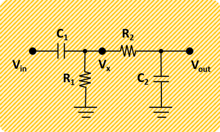
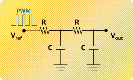
The RC circuit diagram shows the high- and low-pass filters in a cascaded arrangement. The cutoff frequency (rad/s) for the high-pass is ![]() and
and ![]() for the low-pass. In terms of time constants (which will be helpful later with conciseness), we have respectively
for the low-pass. In terms of time constants (which will be helpful later with conciseness), we have respectively ![]() and
and ![]() .
.
For example, a band-pass filter with cutoff frequencies of approximately 0.1 and 2 Hz can be realized with![]() ,
, ![]() ,
, ![]() , and
, and ![]() . Or, using time constants,
. Or, using time constants,![]() and
and ![]() .
.
That’s about it for the analog implementation of a first-order band-pass filter. Let’s see how we can derive the digital version of the same filter and have it ultimately implemented in Python code (at the bottom of this post if you want to skip the technical mumbo jumbo).
Continuous Filter
The first step is to come up with a mathematical representation of the band-pass filter in the analog (continuous) domain. More specifically, as already mentioned in the PID tuning post, let’s work with the Laplace transform (or s-domain), which conveniently turns differential equations into much easier to solve polynomial equations.
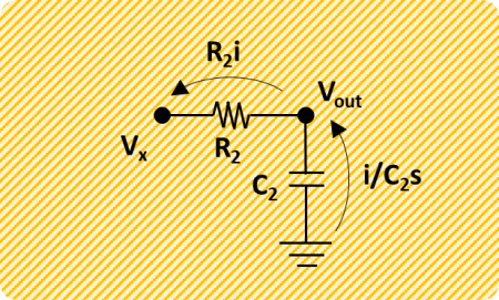
In the case of the RC circuit for the band-pass filter, we want to find the transfer function between the output voltage![]() and the input voltage
and the input voltage![]() . In other words, between the raw and the filtered signals.
. In other words, between the raw and the filtered signals.
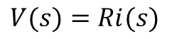
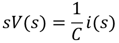
The relationships between voltage and current for the resistor and capacitor are given by:
and
In the s-domain, the derivative operator![]() is “replaced” with the algebraic s operator:
is “replaced” with the algebraic s operator:
and
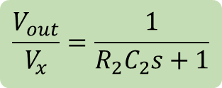
The filter can be separated into two filters (a high-pass and a low-pass), where distinct transfer functions between![]() and
and![]() , as well as between
, as well as between![]() and
and ![]() , can be derived and then combined.
, can be derived and then combined.

Solving the system’s first equation (below) for the current and substituting in the second equation gives:
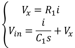

And rearranging as a transfer function:
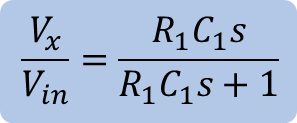
Solving the system’s first equation (below) for the current and substituting in the second equation gives:


And rearranging like the high-pass case:
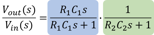
Finally, solving the function for the low-pass filter for![]() and substituting the result in the function for the high-pass filter, will lead to the transfer function of the band-pass filter below (also shown in terms of time constants and descending powers of s):
and substituting the result in the function for the high-pass filter, will lead to the transfer function of the band-pass filter below (also shown in terms of time constants and descending powers of s):

Discrete Filter
The next task is to convert the continuous system to a discrete one. Similarly to the continuous domain, where the derivative operator![]() is represented by the operator s, the discrete domain has the operator z.
is represented by the operator s, the discrete domain has the operator z. ![]() (or 1) corresponds to the current time step discrete value
(or 1) corresponds to the current time step discrete value![]() ,
, ![]() corresponds to the previous value
corresponds to the previous value ![]() ,
, ![]() to the value before the previous one
to the value before the previous one![]() , and so on.
, and so on.
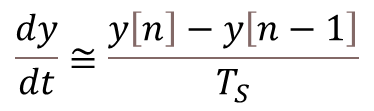
As seen in the post about digital filtering, for a discrete system with sampling period![]() , the derivative of a continuous variable can be approximated by the backward difference below:
, the derivative of a continuous variable can be approximated by the backward difference below:
And in terms of operators, we can write:

Substituting s in the continuous transfer function for the band-pass filter gives the equation in the z-domain below. Note also that, because we are talking about a filter for any type of signal, the voltages were replaced by more general input and output variables.
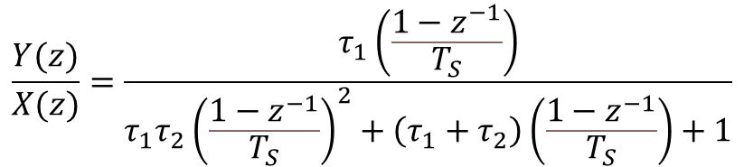
Carrying out the math so we can regroup in terms of descending powers of z, and multiplying both top and bottom by![]() , leads to:
, leads to:

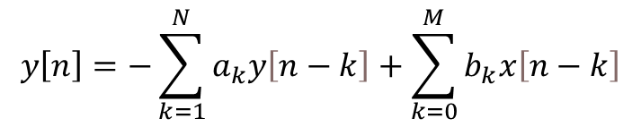
We can then rearrange the z transfer function above to resemble a difference equation:

Where:
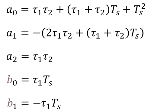
At last, the equation above can be brought to a more useful difference equation form, by replacing the z operators by their corresponding discrete system values:

Python Code for Band-Pass Filter
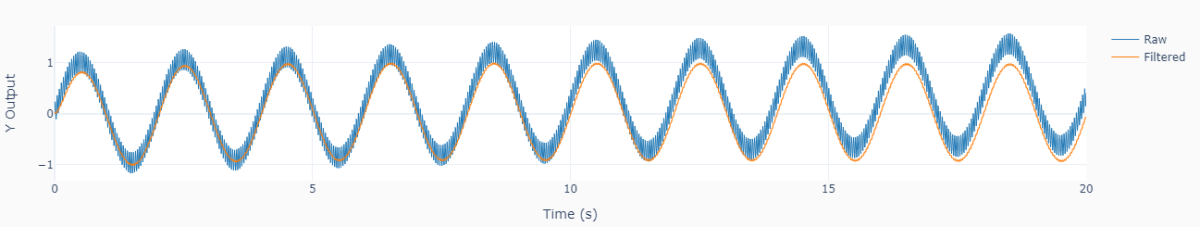
The following Python program implements the digital filter with a fictitious signal comprised of three sinusoidal waves with frequencies 0.01, 0.5, and 25 Hz. The low and high cutoff frequencies of the filter are 0.1 and 2 Hz, therefore allowing only the 0.5 Hz component of the original signal to pass through.
By analyzing the code, it is straightforward to identify the filter coefficients determined in the previous section. The difference equation was implemented in the more general form
where the sets of coefficients![]() and
and![]() are normalized by the coefficient
are normalized by the coefficient![]() of the output
of the output![]() . This approach allows for any type of digital filter to be used in the code, as long as the normalized coefficients are defined.
. This approach allows for any type of digital filter to be used in the code, as long as the normalized coefficients are defined.
# Importing modules and classes
import numpy as np
from utils import plot_line

# "Continuous" signal parameters
tstop = 20  # Signal duration (s)
Ts0 = 0.0002  # Time step (s)
fs0 = 1/Ts0  # Sampling frequency (Hz)
# Discrete signal parameters
tsample = 0.01  # Sampling period for code execution (s)
# Preallocating output arrays for plotting
tn = []
xn = []
yn = []

# Creating arbitrary signal with multiple sine functions
freq = [0.01, 0.5, 25]  # Sine frequencies (Hz)
ampl = [0.4, 1.0, 0.2]  # Sine amplitudes
t = np.arange(0, tstop+Ts0, Ts0)
xs = np.zeros(len(t))
for ai, fi in zip(ampl, freq):
    xs = xs + ai*np.sin(2*np.pi*fi*t)

# First order digital band-pass filter parameters
fc = np.array([0.1, 2])  # Band-pass cutoff frequencies (Hz)
tau = 1/(2*np.pi*fc)  # Filter time constants (s)
# Filter difference equation coefficients
a0 = tau[0]*tau[1]+(tau[0]+tau[1])*tsample+tsample**2
a1 = -(2*tau[0]*tau[1]+(tau[0]+tau[1])*tsample)
a2 = tau[0]*tau[1]
b0 = tau[0]*tsample
b1 = -tau[0]*tsample
# Defining normalized coefficients
a = np.array([1, a1/a0, a2/a0])
b = np.array([b0/a0, b1/a0])
# Initializing filter values
x = np.array([0.0]*(len(b)))  # x[n], x[n-1], x[n-2], ...
y = np.array([0.0]*(len(a)))  # y[n], y[n-1], y[n-2], ...

# Executing DAQ loop
tprev = 0
tcurr = 0
while tcurr <= tstop:
    # Doing I/O computations every `tsample` seconds
    if (np.floor(tcurr/tsample) - np.floor(tprev/tsample)) == 1:
        # Simulating DAQ device signal acquisition
        x[0] = xs[int(tcurr/Ts0)]
        # Filtering signal
        y[0] = -np.sum(a[1::]*y[1::]) + np.sum(b*x)
        # Updating previous input values
        for i in range(len(b)-1, 0, -1):
                x[i] = x[i-1]
        # Updating previous output values
        for i in range(len(a)-1, 0, -1):
                y[i] = y[i-1]
    # Updating output arrays
    tn.append(tcurr)
    xn.append(x[0])
    yn.append(y[0])
    # Incrementing time step
    tprev = tcurr
    tcurr += Ts0

# Plotting results
plot_line(
    [t, tn], [xs, yn], yname=['X Input', 'Y Output'],
    legend=['Raw', 'Filtered'], figsize=(1300, 250)
)
The plot below shows the code output where the low frequency drift and the high frequency noise are almost fully removed from the signal, while the desired component of 0.5 Hz is preserved.