Tag: PID

Motor Position Control with Raspberry Pi

Motor Position Control with Raspberry Pi

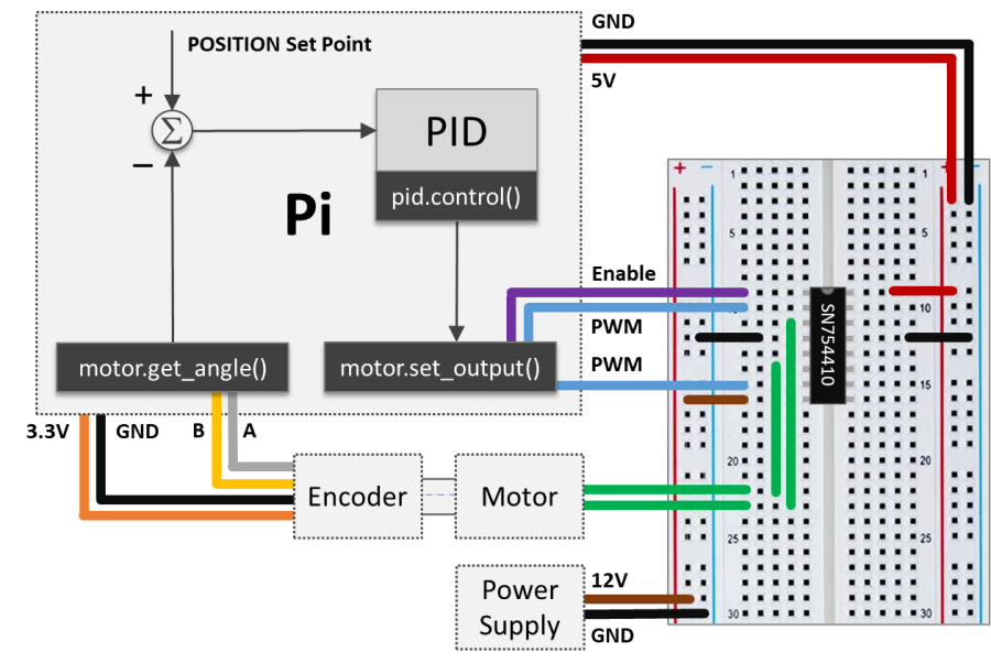
Along the lines of the Motor Speed Control post, let’s reuse some of our Python classes to control the angular position of a DC motor. We’ll also look into how to tune the PID using the Ziegler-Nichols method, as well as different ways to apply a position set point input.

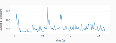
Like before, the starting point is the Raspberry Pi setup that can handle both a PWM output and an encoder input. Unlike the speed control scenario, there’s no need to calculate and filter the speed from the measured angular position.

Most of the work presented in this post was done using the Python code below. It uses the Motor class and the Digital PID class as its building blocks. On my GitHub page, you can find the complete version of this program, a slight variation of it (used for the PID tuning), and all the classes that it uses.

# Importing modules and classes
import time
import numpy as np
from gpiozero_extended import Motor, PID

# Setting general parameters
tstop = 1  # Execution duration (s)
tsample = 0.01  # Sampling period (s)
thetamax = 180  # Motor position amplitude (deg)

# Setting motion parameters
# (Valid options: 'sin', 'cos')
option = 'cos'
if option == 'sin':
    T = 2*tstop  # Period of sine wave (s)
    theta0 = thetamax  # Reference angle
elif option == 'cos':
    T = tstop  # Period of cosine wave (s)
    theta0 = 0.5*thetamax  # Reference angle

# Creating PID controller object
kp = 0.036
ki = 0.379
kd = 0.0009
taupid = 0.01
pid = PID(tsample, kp, ki, kd, tau=taupid)

# Creating motor object using GPIO pins 16, 17, and 18
# (using SN754410 quadruple half-H driver chip)
# Integrated encoder on GPIO pins 24 and 25.
mymotor = Motor(
    enable1=16, pwm1=17, pwm2=18,
    encoder1=24, encoder2=25, encoderppr=300.8)
mymotor.reset_angle()

# Initializing variables and starting clock
thetaprev = 0
tprev = 0
tcurr = 0
tstart = time.perf_counter()

# Running execution loop
print('Running code for', tstop, 'seconds ...')
while tcurr <= tstop:
    # Pausing for `tsample` to give CPU time to process encoder signal
    time.sleep(tsample)
    # Getting current time (s)
    tcurr = time.perf_counter() - tstart
    # Getting motor shaft angular position
    thetacurr = mymotor.get_angle()
    # Calculating current set point angle
    if option == 'sin':
        thetaspcurr = theta0 * np.sin((2*np.pi/T) * tcurr)
    elif option == 'cos':
        thetaspcurr = theta0 * (1-np.cos((2*np.pi/T) * tcurr))
    # Calculating closed-loop output
    ucurr = pid.control(thetaspcurr, thetacurr)
    # Assigning motor output
    mymotor.set_output(ucurr)
    # Updating previous values
    thetaprev = thetacurr
    tprev = tcurr

print('Done.')
# Stopping motor and releasing GPIO pins
mymotor.set_output(0, brake=True)
del mymotor

PID Tuning using Ziegler-Nichols

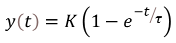
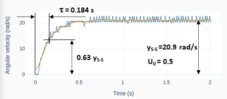
Unfortunately, the PID tuning method presented in the previous post cannot be used to obtain an initial set of controller gains. The first-order approximation used for the speed response doesn’t work for the angular position, since it increases linearly once a steady-state speed is reached. In other words, the DC motor system with position as an output is an integrator of the corresponding system with speed as an output.

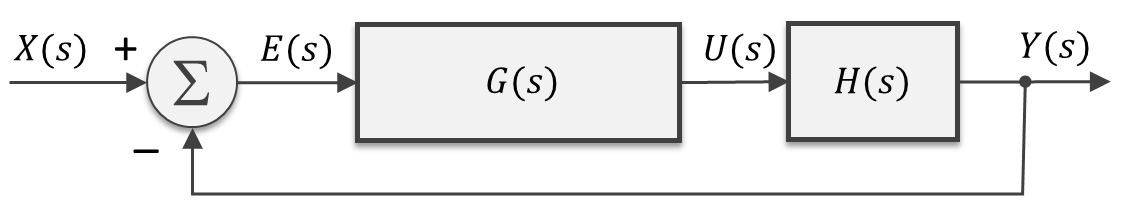
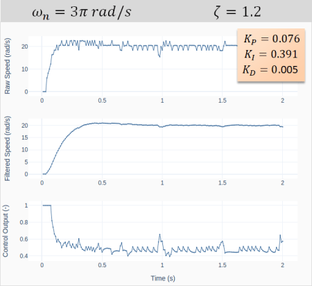
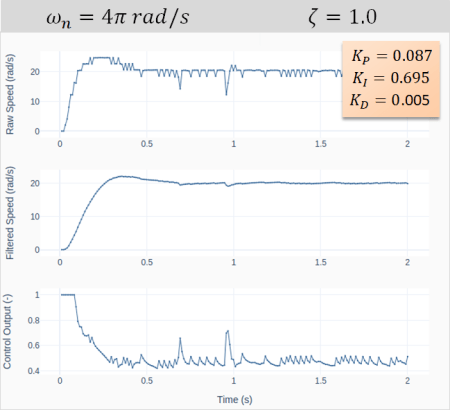
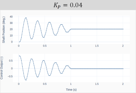
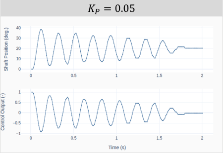
That brings us to the Ziegler-Nichols method, which can be used with a closed-loop system. In our case, the feedback loop is closed on the motor shaft position. The method is based on starting the tuning process only with a proportional gain and then increasing its value, until the closed-loop system becomes marginally stable. I.e., oscillates with a constant amplitude. The four plots below show the response and corresponding controller output for increasing values of.

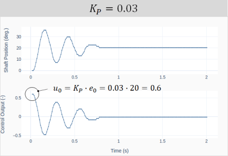
The first question that comes to mind is what should the starting value ofbe. A good guess is based on the size of the step input and the saturation limit of the controller. The very instant the step input is applied, the position error going into the controller is equal to the step size. Therefore, at that moment, the controller output is given by . As shown in the first plot, for , the initial controller output is 0.6 for a step input of 20 degrees. The choice of the step size and the initial proportional gain are such that the controller doesn’t saturate (in our case, 1 is the output limit) and there’s still room to increase the gain without running “too much” into the saturation zone.
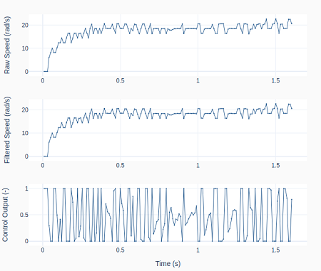
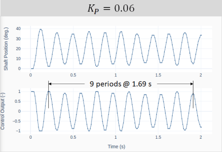
The ultimate proportional gainis achieved when the system oscillates with a constant amplitude. In our example, . Under this condition, the ultimate oscillation period can be extracted from the last plot above and is calculated as.

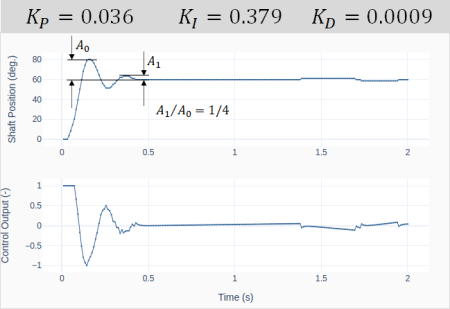
The Ziegler-Nichols method states that for a 1/4 decay ratio of the closed-loop system response, the PID gains are given by:

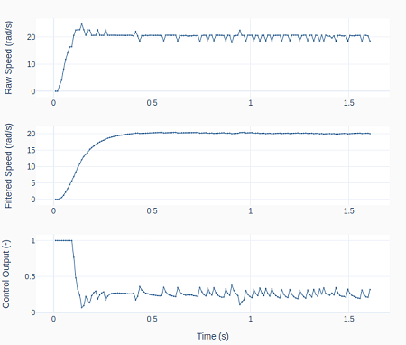
The graph shows the closed-loop response for a shaft position step input of 60 degrees. The PID gains were obtained after substitutingandinto the formulas above.

Observe the 1/4 decay ratio of the amplitude. Also, the fact that the motor position cannot meet exactly 60 degrees causes the integral error to build up, resulting in small position “jumps” around the 1.4 and 1.7 s marks.

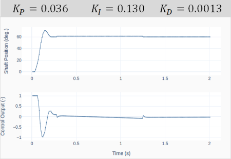
Starting from the gains defined by using the Ziegler-Nichols method, let’s do some manual tuning aiming to decrease the oscillation of the closed-loop response. That can be achieved by decreasing the integral gain and increasing the derivative gain.

The plot on the left shows the system response for values that were obtained after a few attempts. The idea is to later compare the effect of the two sets of gains on the response (when applying different types of position set point inputs).

Sine and Cosine Path Functions

While using step changes to move from one position to another is fine, there are situations where we want the position to follow a pre-determined path. By choosing the right combination of PID gains and characteristics of the path function, it’s possible to greatly improve the tracking ability of the position controller.

In this post let’s take a look at two trigonometric functions (sine and cosine), that can be used to move the motor to a given set point angle and then back to its initial position. By inspecting the code above, we can identify the sine and cosine path functions shown below.

and

By choosing suitable values of the amplitudeand period, the two functions can produce motion paths that have the same set point (maximum) angle and the same motion duration to return to the original angular position.

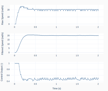
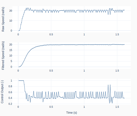
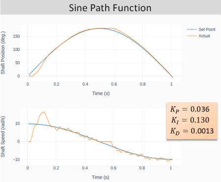
The next two plots show the general closed-loop tracking performance for the sine-based path function, using the two sets of PID gains obtained in the previous section. Notice the more pronounced oscillatory behavior for the more aggressive set of gains. Additionally, due to the nature of the sine-based path, the initial and final speeds are not zero.

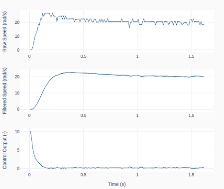
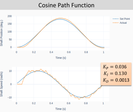
The cosine-based path function on the other hand (shown below) has zero initial and final speeds. That characteristic can greatly reduce the system oscillation, especially at the very beginning of the motion.

Final Remarks

When it comes to position control, the DC motor is usually part of a machine or even a robot, where it is important to understand the dynamic behavior of the complete system. Speed and accuracy are usually conflicting goals that have to be compromised to obtain the best performance of the closed-loop control system. However, having a suitable path function can minimize undesired system oscillation caused by the input excitation (or path).

In future posts we will take a deeper look into path functions, particularly the ones that in addition to having zero end-point speeds also have zero end-point accelerations. Stay tuned!

PID Tuning

PID Tuning

Tuning a PID controller consists of choosing the best values for the proportional, integral, and derivative gains in order to satisfy some performance criteria of the closed-loop system. If we’re able to characterize or model the plant that we want to control, then it’s possible do find the best gains either through direct calculation or through simulation.

If we go back to the day when computers weren’t exactly around and there was no such thing as a digital PID, folks had to come up with methods that could be applied directly to the plant or process. Developed respectively in the 1940s and 50s, the well known Ziegler-Nichols and Cohen-Coon methods were the way to go about PID tuning back then. One problem with those two methods is that they result in a fairly aggressive set of gains that can potentially lead to an unstable (or a reduced stability margin) closed-loop system. That undesired characteristic becomes even more critical when a digital PID is employed.

Because we will be dealing mostly with DC motors, I’ll go over a method where the motor speed response is approximated by a first order system. The identified open-loop system is then used to determine the PID gains for the corresponding closed-loop system. In a future post we will go over characterizing the motor individual plant parameters, thus obtaining a better model.

So, let’s try to keep the math under control and start with characterization of the first-order system.

First-Order System

If we look back at the digital filter post, we can extend the low-pass filter equation to a more general form of the first-order system, given by:

where the steady-state gainis the ratio between system output and input. As seen in that same post,is the response time of the system. By determining those two parameters, the first-order system can be fully characterized.

Closed-Loop System

The block diagram below represents the closed-loop system with a PID controller and our first-order system, the latter now expressed as a differential equation. While technically correct, no one uses a time-based representation of the system as shown in the diagram. Mostly because it is really difficult to work with differential equations whose inputs and outputs are all interconnected in some way.

Thankfully, a pretty smart guy named Pierre-Simon Laplace (1749 – 1827) came up with the Laplace transform. It allows for mere mortals to treat complicated convolution problems involving differential equations as simple algebraic ones. We can then redraw the diagram using the corresponding Laplace transforms, as shown in the more familiar form below.

Because we will be doing some algebraic manipulation let’s use the following transfer function notation:

Where

and

Doing the usual “with a few steps, it can be shown that” the closed-loop system transfer function in our case is:

It has the characteristic equation of a second-order system, with damping ratio(zeta) and natural frequency

or

Where

and

After all this mumbo jumbo, we’re finally getting to a point where, for a given first-order plant (with knownand), we can determine the PID gains,andthat would give us the desired closed-loop response, characterized byand. In other words, by selecting a damping ratio and a natural frequency, we can determine a set of PID gains that make our closed-loop system behave as desired.

PID Gains Selection

If we take a look at the last two equations, there are three unknowns (the PID gains) for two known parameters (and ). A good starting point is to make . That way, we can solve the two following equations, for and.

and

Where:

  • in rad/s is the natural frequency of the closed-loop system. The larger its value the faster the system’s response time. In practical terms, you cannot make this number arbitrarily high since you may run into saturation of the controller output. While, for most applications, short saturation periods are fine, it’s better to keep them at a minimum.
  • is the damping ratio of the closed-loop system. Values close to 1 (critical damping ratio) will keep the oscillations and overshoot to a step input under control. In some closed-loop positioning applications, overshoot isn’t an option. Hence, a damping ratio greater than 1 is required.

Finally, note that the PID gains should always be positive. Therefore,.

DC Motor PID Tuning

It’s time to use the hardware setup and code from the Motor Speed Control post to do some exploration of this PID tuning method. First, a step input is applied to the open-loop motor in order to determine the first order response parametersand.

For our little DC motor, with the Raspberry Pi setup, the steady state gain is 20.9/0.5 = 41.8 rad/s/u. Remember that, in our case, u is the normalized PWM output between -1 and 1. The response time of the open-loop system is 0.184 s.

To improve the parameter extraction, a zero-phase filter was used. The code that automatically determines the parameters from the system response can be found on my GitHub page.

Next step consists of choosing values for the closed-loop system’s natural frequencyand damping ratio. The graphs on the left show the system response to a step input for a natural frequency of 2 Hz () and. Using the last two formulas for the integral and proportional gains

,

with all the values we gathered so far, would result inand. We can observe that the motor now takes 0.11 s to reach the target speed (instead of 0.184 to reach 63% of it). That comes of course at expense of using the full capacity of the PWM with some brief saturation.

The reasoning behind my choice ofandis that I wanted a faster response with limited saturation. 2 Hz was the right amount for that. I also wanted a damping ratio slightly greater than one to avoid any oscillations. At this point you might be asking yourself: why is the closed-loop response showing an oscillatory behavior then! The answer is a combination of:

  • The motor is in fact a second order system, not a first order one as our approximation suggests. So, higher order modes may start showing up in the closed-loop response
  • The PID is discrete, not continuous (as that was the basis for all the deductions above). And we’ve seen that the digitalization of the PID tends to promote a more oscillatory behavior
  • The actual closed-loop system includes the transfer function of a low-pass filter for the motor speed. So, the overall system is not composed only by a PID and a plant, as we initially assumed.

Acknowledging that the choice of gains was fairly straightforward, the resulting closed-loop response is quite good! And we haven’t incorporated the derivative gain yet. While it’s usage is not always necessary, it tends to be quite helpful in the case of closed-loop DC motor control. A good starting point foris a couple of orders of magnitude smaller than the proportional gain. So, after starting with 0.001, I ended up with a value of 0.005. The addition of the derivative term really decreased the overshoot and virtually removed the oscillations.

Finally, the next set of graphs shows the results when choosing different natural frequencies and damping ratios. Notice the effect on the response time, the overshoot and the saturation of the controller output.

Motor Speed Control with Raspberry Pi

Motor Speed Control with Raspberry Pi

Let’s use the Motor class with encoder and the Digital PID class to create a closed-loop speed controller for a DC motor. Those two classes have all the required attributes and methods that we need to program an execution loop for a PID controller with very few lines of code.

The starting point is the Raspberry Pi setup that was used to implement encoder capability into the Motor class. I took the artistic liberty to create the diagram below, where I combine visual elements of the PID loop, the hardware connections, and the class methods used for the I/O between the Pi computer and the physical system.

Going back to the concept of execution loops, the I/O tasks are taken care by the Motor class methods get_angle() and set_output(). The computation tasks happening in between are essentially the shaft speed calculation, low-pass filtering, and PID control action. The Python code below implements the execution loop, where the different elements in the Pi box above can be identified. The complete program, which includes the plotting features, along with the Python module with all necessary classes, can be found on my GitHub page.

# Importing modules and classes
import time
import numpy as np
from gpiozero_extended import Motor, PID

# Setting general parameters
tstop = 2  # Execution duration (s)
tsample = 0.01  # Sampling period (s)
wsp = 20  # Motor speed set point (rad/s)
tau = 0.1  # Speed low-pass filter response time (s)

# Creating PID controller object
kp = 0.15
ki = 0.35
kd = 0.01
taupid=0.01
pid = PID(tsample, kp, ki, kd, umin=0, tau=taupid)

# Creating motor object using GPIO pins 16, 17, and 18
# (using SN754410 quadruple half-H driver chip)
# Integrated encoder on GPIO pins 24 and 25.
mymotor = Motor(
    enable1=16, pwm1=17, pwm2=18,
    encoder1=24, encoder2=25, encoderppr=300.8)
mymotor.reset_angle()

# Initializing previous and current values
ucurr = 0  # x[n] (step input)
wfprev = 0  # y[n-1]
wfcurr = 0  # y[n]

# Initializing variables and starting clock
thetaprev = 0
tprev = 0
tcurr = 0
tstart = time.perf_counter()

# Running execution loop
print('Running code for', tstop, 'seconds ...')
while tcurr <= tstop:
    # Pausing for `tsample` to give CPU time to process encoder signal
    time.sleep(tsample)
    # Getting current time (s)
    tcurr = time.perf_counter() - tstart
    # Getting motor shaft angular position: I/O (data in)
    thetacurr = mymotor.get_angle()
    # Calculating motor speed (rad/s)
    wcurr = np.pi/180 * (thetacurr-thetaprev)/(tcurr-tprev)
    # Filtering motor speed signal
    wfcurr = tau/(tau+tsample)*wfprev + tsample/(tau+tsample)*wcurr
    wfprev = wfcurr
    # Calculating closed-loop output
    ucurr = pid.control(wsp, wfcurr)
    # Assigning motor output: I/O (data out)
    mymotor.set_output(ucurr)
    # Updating previous values
    thetaprev = thetacurr
    tprev = tcurr

print('Done.')
# Stopping motor and releasing GPIO pins
mymotor.set_output(0, brake=True)
del mymotor

Motor Speed Filtering

Now that the Python code is laid out, let’s go over some of its components. The motor shaft speed is calculated as the derivative of the angular position of the shaft using a backward difference formula wcurr = np.pi/180 * (thetacurr-thetaprev)/(tcurr-tprev).

The encoder that’s being used has a resolution of encoderppr=300.8, which corresponds to approximately 360/300.8 = 1.2 degrees. The difference between two consecutive time steps tcurr and tprev is about tsample = 0.01 seconds. That gives us a not so great speed resolution of np.pi/180 * (1.2)/(0.01) = 2 rad/s (or 19 rpm!). As a side note, the speed resolution could be improved by increasing either the encoder PPR or the sampling rate. However the first option might reach the limit of the GPIO zero RotaryEncoder class, while the latter will eventually make the closed-loop system unstable. Therefore a compromise has to be reached given the constraints at hand.

One way reduce the impact of this limitation is to apply a low-pass digital filter to the motor speed signal: wfcurr = tau/(tau+tsample)*wfprev + tsample/(tau+tsample)*wcurr. The graphs below show the raw and the filtered signal as well as the controller output.

On the left, tau = 0 and therefore no filtering is being done. Observe how the controller output bounces between saturation limits. On the right, tau = 0.1, causing the control output to be less erratic, which in turn makes the raw speed more stable. One can also see the “discretization effect” of the 2 rad/s speed resolution on the top row plots.

As discussed in the post Encoder with Raspberry Pi, we cannot use a more accurate sampling period during the execution loop due to the intensive computing resources of the RotaryEncoder class.

However, as shown on the left, having to rely on the command time.sleep(tsample) inside the execution loop, still produces repeatability of the sampling period within 1 ms.

PID Derivative Term Filtering

If you notice in the Python code above, I am also filtering the PID derivative when I created the PID class instance: pid = PID(tsample, kp, ki, kd, umin=0, tau=taupid), where taupid = 0.01 seconds.

If we turn it off by making taupid = 0, we obtain the results on the left, where the controller output shows a bigger oscillation amplitude. However, the effect of turning the derivative term filter off is not as pronounced as the effect of not filtering the motor speed signal.

By comparing all the system responses so far, even though the PID gains were never changed from case to case, the closed-loop system response is changing. Ultimately, by adding low-pass filters, the closed-loop dynamic system is different from its original form without the filters.

PID Saturation and Anti-Windup

As it can be seen in the previous graphs, the PID output is saturating right after the step input. We can observe the effect of PID saturation and the integral term windup (which has been avoided so far) by creating the PID class instance: pid = PID(tsample, kp, ki, kd, umin=-10, umax=10, tau=taupid).

Because the controller output (PWM in the Motor class) is in fact limited between -1 and 1, applying -10 and 10 as the new PID controller limits will effectively turn off the anti-windup feature and cause the integral term to wind up.

The plots on the left show the resulting speed overshoot due to that modification as the actual PWM output is saturated at 1.

Final Remarks

We have been building up our knowledge with the previous posts (namely: Encoder with Raspberry Pi, Digital Filtering, and Digital PID Controller) so we could finally run a DC motor in closed-loop speed control. While this could have been achieved from the very beginning, I believe it was more educational to do it in smaller parts through the use of Python classes.

When building more complex automation systems, having a modularized approach with classes that can be tested and used independently, as well as combined in different ways, will make things much easier to tackle in the long run.