Tag: DC Motor

DC Motor Characterization (2 of 2)

DC Motor Characterization (2 of 2)

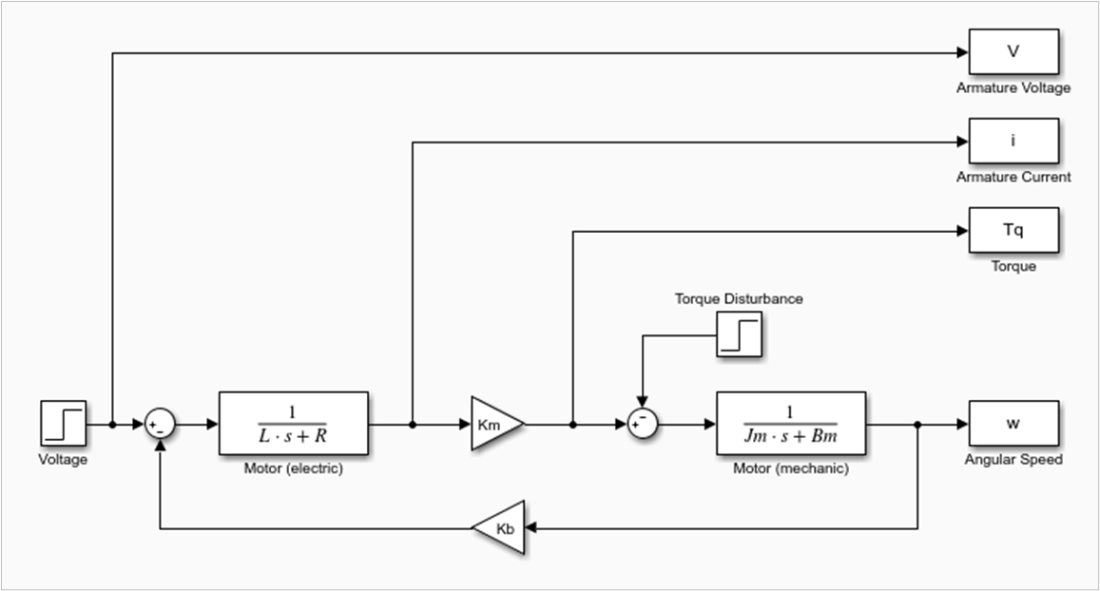
Picking it up from where we stopped in the previous post, let’s see how we can determine the effective moment of inertia, the effective damping and the torque constant for the reduced order model shown in the diagram.

Before we start, it’s a good idea to revisit a typical set of torque/speed curves for a DC motor. They will come in handy to better understand the parameter determination (identification) tests that are explained further down the post.

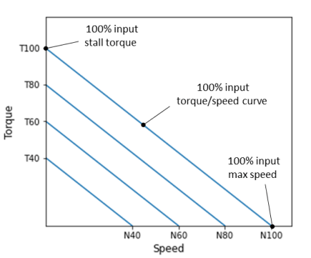
The graph shows torque/speed curves at constant input voltages for a DC motor, for arbitrarily chosen levels of 40, 60, 80 and 100%.

The torque values on the zero-speed y-axis represent the motor stall torque at different input voltages. Conversely, the speed values on the zero-torque x-axis represent the unloaded maximum motor speed, also at different input voltages.

These two special sets of data points will be used to determineandrespectively.

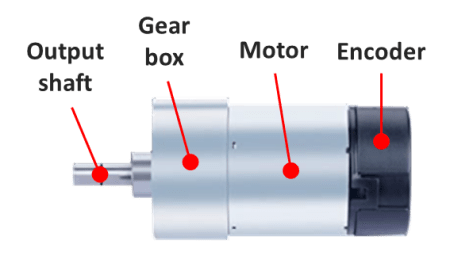
This time around, I’ll use a LEGO Mindstorms EV3 large motor. The basic reason behind such hardware choice is the easiness to build different test fixtures based on the parameter that’s being identified.

Determination of DC Motor Torque Constant
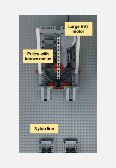
The torque constantcan be determined through a series of torque stall tests with varying motor input levels. The images below show the LEGO fixture that was built to accomplish the task.

The fixture design allows for the motor angular motion to be converted to a linear motion through the pulley system and the Nylon line. Therefore, the torque can be calculated from the measured linear force using the spring gauge.

Since the radius of the large pulley is known, the measured force in N can be converted to a measured torque in N.m.

The low budget gauge accuracy was verified with known masses and proved to be meet the standards of this blog. As a side note, calibration/verification of your measurement gauges should always be a part of any experimental testing!

Because of the nature of the force gauge, where the measurement readings had to be done visually by myself, it wasn’t possible to automate this test. Nonetheless, I used the pyev3 package to create a motor object and interactively set output levels.

It should be noted that the motor input can range between -100 and 100 %. The values are likely PWM duty cycle and seem to have a linear relationship with armature voltage (to which I don’t have access through the EV3 brick).

Finally, the mass of the spring gauge was taking into account when calculating the torque values.

The stall torque was measured for 4 large EV3 motors, where each point on the plot is the average of three torque values calculated from the corresponding force reading.

Four input levels were used, i.e., 40, 60, 80, and 100%. The dashed lines were fitted to the data points for each motor. Now, if we remember from the first test of the previous post that:

Then the slope of each line represents the torque constant in N.m/%. The average value is:

Determination of DC Motor Damping

Similarly to the torque constant determination, four large EV3 motors were used to generate the damping data. This time around however, because no torque load is applied to the motors, no fixture was required for the testing other than my hand holding the motor.

The plot shows the results for the zero-load tests, where each point is the average of three measurements for a given motor. The same input levels of the previous section were used.

If we reference back to the second test of the DC Motor Characterization (1 of 2) post, where:

The slope of the fitted dashed lines represents the speed constant in rad/s/%. The average value is:

Since we already know the value of the torque constant, the damping constant can then be calculated, leading to:

The Python code used to generate the plots and data fits above, as well as the automated test for the determination of the motor speed constant, can be found here.

Determination of DC Motor Inertia

The final parameter to be identified is the effective moment of inertia. As the name suggests, it accounts for the rotor inertia and any rotating masses attached to the output shaft. In the particular case of the EV3 motor, there’s a gearbox between the rotor and the output shaft. Therefore the moment of inertia of all the gears and the effect of the gear ratios will be accounted for, once we determine the effective moment of inertiareduced to the output shaft.

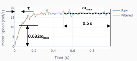
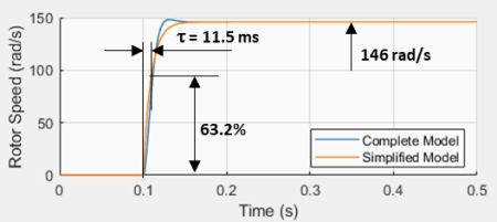
The moment of inertia will be estimated using the third test from the previous post as illustrated on the plot to the left. The idea is to determine the time constantof the approximated first order system and use

to determine since is already known.is the time to reach 63.2% of the steady-state speed value.

Some signal processing was used, as suggested in the graph above. A zero-shift low-pass filter was applied to the motor angular speed signal and thenwas calculated as the median value of the last 0.5 seconds of the signal. With the steady-state speed value in hands, can be easily determined and therefore .

Four different motors were tested at four input levels (40, 60, 80, and 100%), where five measurements were taken at each level. With a median time constantof 0.076 s, and using the the formula above with the already determined , The effective moment of inertia at the motor shaft output is:

Note that the effective moment of inertia is a fairly large number for such a small motor. Remember however that the moment of inertia at the shaft output is proportional to the squared value of the gear ratio. Which means, for our particular LEGO motor, if the gear ratio is for example 1:30, the rotor moment of inertia is 900 times smaller that the value at the gearbox output!

More on Effective Moment of Inertia

Let’s explore what happens if we attach an additional rotating mass to the shaft output, thus modifying the effective moment of inertia. One would expect the response time constant to increase as the rotating inertia increases.

To that end, the original test fixture was modified to accommodate two balanced counter weights. Such setup creates a zero load torque while allowing for different load inertias (by changing the mass of the counter weights).

Just for the sake of this exercise, let’s call the original effective moment of inertia of the LEGO large motor at the output shaft asand the additional inertia due to the counter-weights as . Note that

whereis the total mass of the counter-weights andis the radius of the pulley. The moment of inertia of the pulley is negligible when compared to that of the counter-weights.

Two sets of weights were used, i.e., 0.149 and 0.249 kg with a corresponding moment of inertia of 0.00023 and 0.00045 kg.m2 (the pulley radius is 39.25 mm). Using the formula below with all the known quantities allows us to calculate the time constant of the system with motor plus counter-weights.

In our case, the calculated values ofare 0.086 and 0.098 s. Running the test shown on the left, with four different motors and four different output levels, in fact produced measured values within +/- 3% of the corresponding calculated ones!

DC Motor Model Confirmation

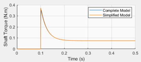
It’s always a good idea to check whether the motor characterization parameters can be used to build a model that represents the actual system behavior. To do that, a set of counter-weight masses that haven’t been tested during the characterization was chosen, resulting in the following motor model.

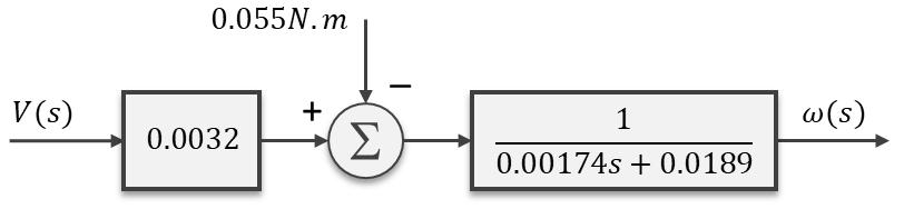
Where the load torque due to the uneven counter-weight masses is 0.055 N.m and the effective inertia is 0.0014 + 0.00034 = 0.00174 kg.m2. The plot on the left shows good agreement between the actual LEGO fixture test results and the Simulink simulation of the reduced-order model above, for a 70% duty-cycle step input.

DC Motor Characterization (1 of 2)

DC Motor Characterization (1 of 2)

In this first of two posts, we’ll go over the simplifications of the equations that govern the dynamic behavior of a DC motor. By doing so, we should be able to use a non-intrusive and fairly straightforward approach to determine the parameters that characterize the motor from a control systems stand point.

While this might get a bit arid at times, I’ll try to keep it interesting by using some real motor parameters and Simulink to show the impact of the simplifications as we move towards our final dynamic system equation. Let’s start with the well known coupled differential equations (which are essentially a mathematical representation) for the electric motor:

Where (in SI units, for good measure):

By applying the Laplace transformation to the equations above and rearranging them in a way that they are solved for the angular velocity and current, we get:

and therefore

The rearranged equations can then be represented in the form of a block diagram, which will come in handy when we talk about the model simplification. Also, note the negative “feedback” nature of the back EMF term(which makes the rotor speed inherently stable to small disturbances in the load torque).

The DC motor has two time constants associated with its dynamic behavior. The electrical time constant(directly obtained from one of the first-order blocks in the diagram) and the mechanical time constant, which is not so intuitive and we’ll see later where it comes from.

Especially for smaller motors, the electrical time constant is substantially faster than the mechanical time constant. That is generally accompanied by, which means that the corresponding inductance term in the first-order block can be neglected. The block diagram of the resulting system is shown next.

It’s time to put some numbers into these two models and observe how they behave when simulated using Simulink. In order to do that, I found myself a motor data sheet for permanent magnet DC motors from Moog. These tend to be very high end components when compared to the DC motors I’ve been using in my previous posts. I.e. they are designed for a more professional application. Not for the “DIY-finite-budget-hobbyist”, like myself!

With that said, I chose the smallest and the largest motors from the catalog, whose parameters are summarized below:

C23-L33-W10C42-L90-W30
Lengthmm85229
Diametermm57102
Armature VoltageV (DC)1290
Rated CurrentA4.755
Rated Speedrad/s492159
Rated TorqueN.m0.052.26
Friction TorqueN.m0.020.17
Torque Constant ()N.m/A0.01870.5791
Back EMF Constant ()V/rad/s0.01910.5730
Armature Resistance ()Ohm0.601.45
Armature Inductance ()H0.35e-35.4e-3
Rotor Inertia ()kg.m21.554e-52.189e-3
Damping Coefficient ()N.m/rad/s1e-56.8e-4
Electrical Time Constant ()ms0.583.72
Mech. Time Constant ()ms25.79.54

Taking a closer look at the last two rows, the electrical time constant of the smaller motor is significantly faster than its mechanical time constant, especially when compared to the larger motor. We will see how that plays out in a bit.

Also, for the simulation, the two inputs are the armature voltage and the load (or disturbance) torque, the latter accounting for the friction torque as well. The outputs are shown in the Simulink model picture below. The armature current and angular speed are the ones of most interest for checking the validity of the model against the data sheet values. In other words, when running the model with only voltage and torque as inputs, everything else should “fall in place”, matching the table data.

Small DC Motor Simulation Results

The plots show the simulation results for a step response with the armature voltage (12 V) and rated torque (0.05 N.m) for the small C23-L33-W10 motor. Two Simulink models were used: the complete model (shown above) and the simplified one (not shown here). Both can be found on my GitHub page.

The first takeaway is that the final rotor speed and armature current agree well with the corresponding rated values in the table. Also, the response time of 25.6 ms correlates fairly well with what is, in this particular case, the mechanical response time in the table.

While the simulated steady-state rotor speed is very close to the table value (502 vs 492 rpm), the armature current correlation is not so stellar (4.0 vs. 4.75 A) yet still satisfactory. It should be noted that the table values are probably obtained from actual motor tests or from a more sophisticated model.

The second takeaway is that the reduced order model produces virtually the same results as the complete model.

Large DC Motor Simulation Results

The large motor C42-L90-W30 simulation results show that, when the electrical and mechanical time constants are comparable, the simplified model cannot capture the dynamic behavior of the motor, as it was the case with the small motor.

However, the steady-state values still correlate fairly well with the published table values. A rotor speed of 146 rad/s vs. 159 rad/s, and an armature current of 4.37 A vs. 5 A.

As alluded to in the previous case, even the complete model used in the simulation is still an approximation when it comes to accurately describing the behavior of the DC motor.

Simplified DC Motor Model

With the simulation results in mind, we can use the simplified (or reduced order) model to describe the dynamic response of the types of DC motors that I’ll be dealing with throughout my blog.

From the block diagram it’s possible to write:

And rearranging:

Doing the inverse Laplace Transform to put in back in differential equation form:

or

Where:

As a quick note, if we take a closer look at the reduced model, we can identify the mechanical time constant, in the particular case where there are no additional rotating inertias reduced to the rotor shaft.

At this point, the motor can be characterized if we determine the values for,and. There are three non-intrusive tests that can be done with an actual motor, from which the three aforementioned parameters can be extracted.

The first test is a torque stall test () which reduces our last differential equation to:

From whichcan be determined for a given input voltage and the corresponding load torque that causes the DC motor to stall.

The second test is a steady-state test () with no load torque, which gives us:

Sinceis known from the previous test and the angular velocity can be measured for a given input voltage, the parametercan therefore be determined.

The third test is a transient step-input test with no load, which reduces our simplified equation to:

By measuring the response time of the first-order system,can be finally determined (sinceis already known at this point).

Final Remarks

We have seen how it’s possible to determine, or better said estimate, the main parameters , andfor the reduced order model of a DC motor. This can be accomplished without having to disassemble the motor to measure the rotor moment of inertia, or having a more sophisticated electrical measurement setup to determine the armature inductance.

The three tests described above can be performed on a simple test bench. Part 2 of this post will go over an experimental setup with the LEGO EV3 large motor and some automated testing using the pyev3 python package. Stay tuned!

Encoder with Raspberry Pi

Encoder with Raspberry Pi

An encoder or, more specifically, a rotary incremental encoder is a device that can be used to determine incremental changes of the angular position of a rotating shaft. One of the possible hardware constructions is based on a slotted disk attached to the shaft and a pair of optical sensors with a physical offset. The detection of “dark/bright” transitions, as the shaft rotates and the slots pass in front of the sensors, is converted by an electronic circuit into two pulse trains that have a phase shift of 90 degrees between them.

The two signals that are generated by the encoder have to be then processed by a DAQ device, so that the angular increment (or decrement) of the shaft can be determined by “counting the high/low edge transitions” of the two signals. Some DAQ devices have a hardware implementation to deal with encoder signals, thus allowing for much higher shaft speeds. As it is the case of a LabJack.

The Raspberry Pi, on the other hand, doesn’t have the capability to deal with pulse train inputs via hardware. Therefore, it has to rely on a software implementation to do the “edge counting”. We will focus on the class RotaryEncoder in GPIO Zero, which is quite good and very straightforward to use.

To follow along the contents of this post, you may want to review my previous post (H-Bridge and DC Motor with Raspberry Pi), since a motor with an integrated encoder will be used in the examples and, by the end, we will expand the Motor class by adding encoder input capability to it.

From a nomenclature stand point, encoders that produce a pair of square waves (pulse trains) with a 90-degree phase shift are also known as quadrature encoders. However, to take full advantage of this type of encoder, i.e., count all 4 edge transitions during the rotation through one marker (or slot), a hardware-based edge detection is usually required. So, an encoder disc with 45 slots would give a count of 180 effective pulses per revolution (PPR) for a resolution of 2 degrees (360/180). When using a software-based edge detection, the same encoder would have 45 PPR and a resolution of 8 degrees.

The figure below shows typical connections for a Raspberry Pi. Note that the A and B phases are interchangeable. If the pulse count is decreasing when you’re expecting a positive rotation, just swap the connections of the phase wires.

Checking the PPR of the Encoder

After the encoder is connected to the Pi, as shown above, you can use the following Python code to check if the number of Pulses Per Revolution is what you’re expecting. A couple of things will factor into the PPR value.

If the motor has a gear box, the “advertised” PPR value might be incorrect. First of all, understand if the number refers to the quadrature-based value or the marker-based value. Then check if the number is taking into account the gear ratio of the box.

In my case, I am using a motor with a 16 PPR encoder (advertised as a 64 based on a full quadrature implementation) and a gear ratio of 18.8:1. That gives a value of 16 x 18.8 = 300.8 PPR. Ultimately, you can use the sample program below and turn the output shaft by hand to see what you get!

# Importing modules and classes
import time
import numpy as np
from gpiozero import RotaryEncoder

# Assigning parameter values
ppr = 300.8  # Pulses Per Revolution of the encoder
tstop = 20  # Loop execution duration (s)
tsample = 0.02  # Sampling period for code execution (s)
tdisp = 0.5  # Sampling period for values display (s)

# Creating encoder object using GPIO pins 24 and 25
encoder = RotaryEncoder(24, 25, max_steps=0)

# Initializing previous values and starting main clock
anglecurr = 0
tprev = 0
tcurr = 0
tstart = time.perf_counter()

# Execution loop that displays the current
# angular position of the encoder shaft
print('Running code for', tstop, 'seconds ...')
print('(Turn the encoder.)')
while tcurr <= tstop:
    # Pausing for `tsample` to give CPU time to process encoder signal
    time.sleep(tsample)
    # Getting current time (s)
    tcurr = time.perf_counter() - tstart
    # Getting angular position of the encoder
    # roughly every `tsample` seconds (deg.)
    anglecurr = 360 / ppr * encoder.steps
    # Printing angular position every `tdisp` seconds
    if (np.floor(tcurr/tdisp) - np.floor(tprev/tdisp)) == 1:
        print("Angle = {:0.0f} deg".format(anglecurr))
    # Updating previous values
    tprev = tcurr

print('Done.')
# Releasing GPIO pins
encoder.close()

Motor Class with Encoder

The following diagram expands upon the motor setup from the post (H-Bridge and DC Motor with Raspberry Pi). Just as before, we’re using the SN754410 half-bridge chip to set the motor output. But this time around, we can use the encoder to measure the actual shaft angular position and speed.

The Motor class from the post mentioned above can be updated by doing a few modifications to incorporate the rotary encoder.

Besides some new attributes (or properties) used to handle the encoder parameters and its object, two new methods were added: get_angle(), which returns the current encoder angular position in degrees, and reset_angle(), which resets the encoder angle to zero (a handy functionality to have, since we’re using an incremental encoder).

The updated and fully commented class, as well as the rest of the code in this post, can be found on my GitHub page. Also, if you haven’t done it already, I strongly encourage installing VS Code on Raspberry Pi.

Sinusoidal Motor Excitation

The Python program below uses the updated Motor class to run the DC motor with a sinusoidal excitation. Now that we have the encoder capability added to the class, it is possible to measure the angular position of the shaft and calculate its angular velocity. If you’re using VS Code, you must run the code in a terminal instead of an interactive window. The interactive session really competes with the code for CPU resources.

# Importing modules and classes
import time
import numpy as np
from utils import plot_line
from gpiozero_extended import Motor

# Assigning parameter values
T = 2  # Period of sine wave (s)
u0 = 1  # Motor output amplitude
tstop = 2  # Sine wave duration (s)
tsample = 0.01  # Sampling period for code execution (s)

# Creating motor object using GPIO pins 16, 17, and 18
# (using SN754410 quadruple half-H driver chip)
# Integrated encoder is on GPIO pins 25 and 25
mymotor = Motor(
    enable1=16, pwm1=17, pwm2=18,
    encoder1=24, encoder2=25, encoderppr=300.8)
mymotor.reset_angle()

# Pre-allocating output arrays
t = []
theta = []

# Initializing current time step and starting clock
tprev = 0
tcurr = 0
tstart = time.perf_counter()

# Running motor sine wave output
print('Running code for', tstop, 'seconds ...')
while tcurr <= tstop:
    # Pausing for `tsample` to give CPU time to process encoder signal
    time.sleep(tsample)
    # Getting current time (s)
    tcurr = time.perf_counter() - tstart
    # Assigning motor sinusoidal output using the current time step
    mymotor.set_output(u0 * np.sin((2*np.pi/T) * tcurr))
    # Updating output arrays
    t.append(tcurr)
    theta.append(mymotor.get_angle())
    # Updating previous time value
    tprev = tcurr

print('Done.')
# Stopping motor and releasing GPIO pins
mymotor.set_output(0, brake=True)
del mymotor

# Calculating motor angular velocity (rpm)
w = 60/360 * np.gradient(theta, t)

# Plotting results
plot_line([t, t, t[1::]], [theta, w, 1000*np.diff(t)], axes='multi',
          yname=[
              'Angular Position (deg.)',
              'Angular velocity (rpm)',
              'Sampling Period (ms)'])

Once the code finishes running you should get the graph on the bottom left in a web browser page, assuming you ran it in a VS Code terminal. Differently from my other execution loops, I force an execution “pause” by using the command time.sleep(tsample) inside the loop.

By taking that approach, at the expense of a more accurate sampling period, I free up kernel resources to process other interruptions, such as the very CPU-intensive ones coming from the RotaryEncoder. The object is now capable of detecting all the edge transitions coming from the physical encoder, minimizing the number of missed events.

Taking a closer look at the derivative of the angular position (or the velocity) we can detect some fluctuations that are probably due to missed edge counts. The faster the shaft turns, the more likely that is to happen. In our case, 300 PPR at 400 rpm gives 300 x 400 / 60 = 2000 pulses per second. And because the algorithm inside the RotaryEncoder class has to detect all four edge transitions within a pulse, that puts us at 8000 events/sec (or 125 μs/event). Even though the computer is running individual calculations at the nanosecond level, there are many calculations going on inside the algorithm alongside other synchronous tasks. So 125 μs is probably cutting it close.

Still analyzing the results, the sinusoidal PWM excitation will roughly produce a sinusoidal current input to the motor. Since it is the torque, not the angular velocity, that is proportional to the input current, the speed trace will deviate somewhat from the shape of an actual sine wave. That is also quite apparent on the angular position trace, which should be a cosine wave. The deviations with respect to the expected trace shapes are caused mainly by torque being consumed to overcome friction losses in the initial motion and the response time of the motor itself, as a dynamic system.

That is the inherent behavior of this open-loop system. Now that we have the elements in place, by adding the capability to measure the system output, in future posts we’ll explore what can be done by closing the loop on the angular position of the motor shaft.

H-Bridge and DC Motor with Raspberry Pi

H-Bridge and DC Motor with Raspberry Pi

An H-bridge is an electronic circuit that can switch the polarity of the voltage applied to a load. In our case the load is an electric DC motor that is capable of rotating forward and backward. By using a PWM as an input to the system defined by the H-bridge and the motor, we can go from the digital to the analog domain, similarly to what we did with the Raspberry Pi DAC. In this case however, the motor replaces the RC filter and the output is a continuous motor torque/speed instead of a voltage value.

Looking at the bottom half of the diagram introduced in Analog-to-Digital Conversion, the power amplification stage is integrated into the H-bridge and the actuator is the motor. Together they constitute a digital-to-analog converter in a broader sense.

Since the Pi has a limited power output capability, the amplification stage is achieved with an external power supply or a set of batteries that can produce both the higher voltage and current required by a DC motor application. For this post, I’ll use a variable DC power supply set to 12 V and a small DC motor with an integrated encoder. While the encoder won’t be required at this point, it will be used in future posts. And last but not least, there’s the H-bridge, which can be in a single IC chip or part of an IC board. The two types will be considered for some Python code running on a Raspberry Pi 4B.

SN754410 quadruple half-H driver (chip)

The Texas Instruments SN754410 can be used as 4 half-H drivers or 2 H-bridge drivers, depending on the input configuration. The latter can be used to independently control two DC motors with forward and backward rotation. The figure below shows the pins on the chip and the corresponding GPIO pins on the Raspberry Pi.

For a single motor, in addition to the 5V and GND pins, only 3 GPIO pins are required. Unlike the DAC with RC filters, a much lower PWM frequency can be used for the DC motor. Therefore, any 3 GPIO pins can be chosen since the software-implemented PWM at 100 Hz is sufficient.

The breadboard diagram illustrates the wiring for the DC motor control. For example, the Enable signal can be connected to GPIO16, while PWM Forward and PWM Backward could be connected respectively to GPIO17 and GPIO18. The forward speed of the motor is adjusted through the duty cycle of the PWM Forward signal. Correspondingly, the backward speed uses the PWM Backward signal.

Later on in this post, I will go over a Python Class where the three signals can be used to easily set the motor rotation (in an open-loop fashion for now).

L298 dual H-bridge motor speed controller (board)

Another option is to use an IC board which avoids the need of a breadboard and can therefore be used in a more permanent DIY setup. Most importantly, the reason I chose this particular board is that it has a fundamental difference in how the forward and backward rotation is implemented, when compared to the SN754410 chip.

While the wiring is very similar to the previous setup, by taking a closer look (based on the wiring color scheme), you will notice a different number of Enable and PWM signals. This board has 2 Enable signals and only 1 PWM signal. Rotation direction is now controlled with Enable Forward and Enable Backward, while speed is adjusted with a single PWM duty cycle.

Python Motor Class

Even though GPIO Zero has a Motor Class, the class is not ideal for applications where the motor output speed has to continuously transition between forward and backward rotation direction. The Motor Class implemented in the code below allows for that behavior. Additionally, by coding the class from scratch, we can see how the enable and PWM signals are used, as well as how to accommodate for the two types of wiring setup.

If you have been following along on my blog, in one of my previous posts (VS Code on Raspberry Pi) I encourage the creation of a folder dedicated to your Python modules. With that said, this code should be saved in a module named gpiozero_extended.py alongside utils.py in the /home/pi/python/modules folder on your Raspberry Pi. Also, the fully commented Class can be found on my GitHub page.

from gpiozero import DigitalOutputDevice, PWMOutputDevice


class Motor:

    def __init__(self, enable1=None, enable2=None, pwm1=None, pwm2=None):

        # Identifying motor driver type and assigning appropriate GPIO pins
        if pwm1 and pwm2:
            # Driver with 1 enable and 2 PWM inputs
            # Example: SN754410 quadruple half-H driver chip
            if not enable1:
                raise Exception('"enable1" pin is undefined.')
            self._dualpwm = True
            self._enable1 = DigitalOutputDevice(enable1)
            self._pwm1 = PWMOutputDevice(pwm1)
            self._pwm2 = PWMOutputDevice(pwm2)
        elif enable1 and enable2:
            # Driver with 2 enables and 1 PWM input
            # Example: L298 dual H-bridge motor speed controller board
            if not pwm1:
                raise Exception('"pwm1" pin is undefined.')
            self._dualpwm = False
            self._enable1 = DigitalOutputDevice(enable1)
            self._enable2 = DigitalOutputDevice(enable2)
            self._pwm1 = PWMOutputDevice(pwm1)
        else:
            raise Exception('Pin configuration is incorrect.')
        # Initializing output value
        self._value = 0

    def __del__(self):

        # Releasing GPIO pins
        if self._dualpwm:
            self._enable1.close()
            self._pwm1.close()
            self._pwm2.close()
        else:
            self._enable1.close()
            self._enable2.close()
            self._pwm1.close()

    @property
    def value(self):
        return self._value

    @value.setter
    def value(self, _):
        print('"value" is a read only attribute.')

    def set_output(self, output, brake=False):

        # Limiting output
        if output > 1:
            output = 1
        elif output < -1:
            output = -1
        # Forward rotation
        if output > 0:
            if self._dualpwm:
                self._enable1.on()
                self._pwm1.value = output
                self._pwm2.value = 0
            else:
                self._enable1.on()
                self._enable2.off()
                self._pwm1.value = output
        # Backward rotation
        elif output < 0:
            if self._dualpwm:
                self._enable1.on()
                self._pwm1.value = 0
                self._pwm2.value = -output
            else:
                self._enable1.off()
                self._enable2.on()
                self._pwm1.value = -output
        # Stop motor
        elif output == 0:
            if brake:
                if self._dualpwm:
                    self._enable1.off()
                    self._pwm1.value = 0
                    self._pwm2.value = 0
                else:
                    self._enable1.off()
                    self._enable2.off()
                    self._pwm1.value = 0
            else:
                if self._dualpwm:
                    self._enable1.on()
                    self._pwm1.value = 0
                    self._pwm2.value = 0
                else:
                    self._enable1.on()
                    self._enable2.on()
                    self._pwm1.value = 0
        # Updating output value property
        self._value = output

The following example creates a motor object and runs a sinusoidal excitation with an amplitude of 1 for one full period. If you execute the program, you will notice that the direction of the motor rotation changes as the sign of the sine wave changes.

# Importing modules and classes
import time
import numpy as np
from gpiozero_extended import Motor

# Assigning parameter values
T = 4  # Period of sine wave (s)
u0 = 1  # Motor output amplitude
tstop = 4  # Sine wave duration (s)
tsample = 0.01  # Sampling period for code execution (s)

# Creating motor object using GPIO pins 16, 17, and 18
# (using SN754410 quadruple half-H driver chip)
mymotor = Motor(enable1=16, pwm1=17, pwm2=18)

# Initializing current time stamp and starting clock
tprev = 0
tcurr = 0
tstart = time.perf_counter()

# Running motor sine wave output
print('Running code for', tstop, 'seconds ...')
while tcurr <= tstop:
    # Getting current time (s)
    tcurr = time.perf_counter() - tstart
    # Doing I/O every `tsample` seconds
    if (np.floor(tcurr/tsample) - np.floor(tprev/tsample)) == 1:
        # Assigning motor sinusoidal output using the current time stamp
        mymotor.set_output(u0 * np.sin((2*np.pi/T) * tcurr))
    # Updating previous time value
    tprev = tcurr

print('Done.')
# Stopping motor and releasing GPIO pins
mymotor.set_output(0, brake=True)
del mymotor

DC Motor Remarks

If you’re using a motor with an integrated gear box and try some low output values with the motor object, you’ll notice that there’s a dead band where there’s no speed response as the sign changes around small duty cycle values. That happens because it is the DC motor torque (not the angular velocity) that is proportional to the input current (or very simplistically the PWM duty cycle). For small duty cycle values, the torque is being used to overcome the friction losses in the motor bearings and the gear box before the output shaft starts to turn.

There are several low-budget small DC motors that can be purchased online, usually with a wide range of gear ratios for the same overall packaging constraints. There should be an output shaft speed / torque combination that meets your project requirements. Keep in mind that the SN74410 has a limit of 1 Ampère per driver, which might affect the output that can be achieved. Board controllers are generally rated at much higher currents (5 A and above). The power supply capability should also be taken into account, by the way.

Finally, as I mentioned at the top, a motor with an integrated encoder will become essential if we want to incorporate the angular position of the output shaft into the Motor Class. That will enable closed-loop control of the motor speed and/or angular position, making for a good automation example.