Category: Engineering

Digital PID Controller

Digital PID Controller

Closed-Loop PID (Proportional Integral Derivative) controllers are quite popular when it comes to regulating a dynamic system that has to follow a desired set point. When compared to other types of controllers, it has the advantage of requiring little to no knowledge about the system plant for it to be designed successfully.

Before we start, the idea of this post isn’t to go over the theory of control systems. The goal is to talk about some of the characteristics of a PID controller and how to go about implementing a discrete (or digital) one with some additional features to make it more robust. In the end, we will have a Python class that represents a PID, which can be used in an execution loop to control a process or a dynamic system.

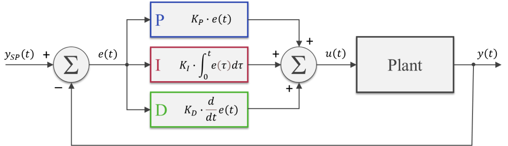
The diagram below illustrates a closed-loop system, where all the signals are represented in the time domain. The three terms of the PID are shown separately, where the controller output valueis the sum of the individual term contributions. The regulation of the plant outputto the desired set point valueis achieved as the controller continuously brings the errorbetween the set point and the plant output to zero.

The PID gains,andcan be tuned so that the closed-loop dynamic behavior ofmeets the desired response requirements. In broad terms, the proportional term reacts directly to the current value of the error between set point and desired output. Usually, the proportional term by itself cannot bring the error to zero (since it relies on the existence of an error to produce a controller output). That’s where the integral term comes into the picture: because it takes into account the accumulated error (or the integrated error) it will compensate the smallest deviations. Over time the accumulation of the deviation will be large enough to cause a controller output. The proportional and integral terms combined can bring the error to zero (for a steady state input) for most dynamic systems.

The derivative term reacts to the rate of change of the error and can be effective for sudden set point changes, by helping reduce the response overshoot. In practical applications, using a derivative term can be tricky due to its sensitivity to noise that’s typically present in the measurement of the plant output.

As a side note, the plots throughout this post were generated using MATLAB and Simulink, where the corresponding m-files and Simulink model can be found on my GitHub page. I should emphasize that I did spend some time exploring and trying to use the Python Control Systems package. However, nothing can beat Simulink when it comes to quickly representing and simulating dynamic systems. Especially when non-linearities are being modelled. Spending $100 on that MATLAB student license might be something to think about.

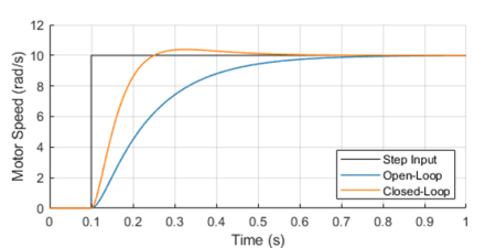
One way to analyze the performance of a control system (in our case a PID controller) is by measuring the closed-loop system’s response to a step change of the set point.

Because in future posts we will be doing closed loop control of small low-budget DC motors, let’s use as a plant a somewhat fictitious motor with an integral gear box. The plot shows the closed-loop system response in contrast with the open-loop response.

The controller output (armature voltage), as well as the individual contribution of each of the PID terms, is also shown. Observe how the proportional and derivative terms go to zero as the response approaches its steady-state value, leaving the integral term in charge of keeping the errorat zero.

It’s important to mention that both the open-loop as well as the closed-loop responses end up at the same final armature voltage of 2.8 V.

For our DC motor model, the armature voltage required to produce a motor speed output of 10 rad/s without any external load is 2.8 V. In the case of the open-loop system, I use that knowledge to apply a step input of 2.8 V to the motor. On the other hand, the step input to the closed-loop system is in fact the desired speed output of 10 rad/s. The PID controller will apply whatever armature voltage is needed to follow the speed set point, even when the manufacturing variability of the motor or other sources of error are present. That’s the first takeaway that most people working with control systems are very familiar with. The second point I want to make is that the improved response time, compared to the open-loop system, can only be achieved because the controller has an excess output capability (up to 12 V in our motor model) that can be tapped into at the moment of the step change.

Without getting into stability margins, the closed-loop system can be just as fast as you want. The issue at hand becomes how much do you want to “oversize” your system so it can obtain that stellar dynamic response. Understanding you engineering requirements is key when choosing the right hardware “size” for the desired closed-loop system behavior.

Discrete PID Implementation

The most basic digital PID implementation can be obtained from taking the derivative of the controller output equation

and using backward difference (with sampling period) to approximate the derivatives. The difference equation below can be obtained by following the steps shown here.

This implementation has two notable advantages:

  • Because the previous output value is taken into account for the output calculation, the controller can be seamlessly started from an open-loop condition by assigning the current open-loop output value to the very first .
  • The PID gains,andobtained from the design of a continuous controller are still valid in its discrete representation (provided a fast enough sampling periodis used).

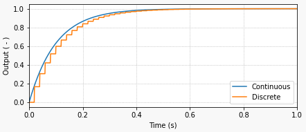
The graphs below show the closed-loop response of the analog plant (DC motor) as well as the corresponding output of the discrete controller for a sampling period of 0.01 and 0.005 seconds. The equivalent analog controller using the same PID gains is also shown as a reference. Although not on the graphs, the discrete PID with a sampling period of 0.001 seconds produces virtually the same response as the continuous one.

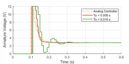
As it can be seen in the graphs, the lower sampling period caused the plant output to oscillate. Further increasingwould increase the amplitude of the oscillations, eventually making the system unstable. This well known behavior is caused by the discretization of the controller, where the plant basically behaves in an open loop fashion in between sample points. Even though this problem can be approached mathematically, tackling it using a simulation tool can provide valuable insight on the compromises between sampling period and PID gains, during the initial design of the controller.

Before we put our digital PID into a Python class, let’s go over a few features that can make the controller more robust for practical applications.

Saturation and Anti-Windup

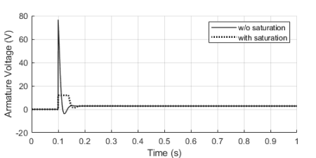
If we were to use some very aggressive gains for our motor PID controller, the step response could be further improved as shown with the solid trace below. You’ll also notice an unpractical armature voltage spike over 60 V! In reality, the controller output will saturate at its maximum (or minimum) output capability, in our case 12 V, producing the dotted line traces instead.

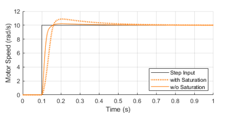
Once the controller output is saturated, the integral term compensation keeps increasing in an attempt to reduce the accumulated error. By the time the controller “comes back” from the saturation state, the integral term is “wound-up”, resulting in an overshoot of the response, as it can be seen by contrasting the dotted and solid orange lines above.

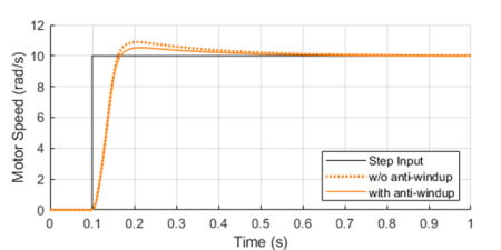
By implementing anti-windup logic in the discrete controller, the overshoot caused by potential saturation can be reduced, as shown on the left.

The basic idea is to turn off the integral term of the PID (as we’ll see in the Python class at the end) every time an upper or lower saturation limit is exceeded. This is a common improvement used in digital PID controllers.

Feed-Forward and Derivative Term Filtering

Another useful improvement that can be made to our digital PID is to allow for a feed-forward signalin its implementation. The feed-forward term reduces the contribution of the controller output signal , making the system less susceptible to noise in the measurement of the plant output used to calculate the error.

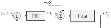
While not always possible, in some special situations, we can pre-calculate the feed-forward signal as a function of time and add it to controller output as shown in the block diagram. Typical applications involve a known “control path” such as a robotic manipulator (with pre-programmed motion paths) or a vehicle’s cruise control (on a highway with known topology).

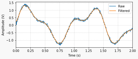
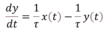
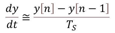
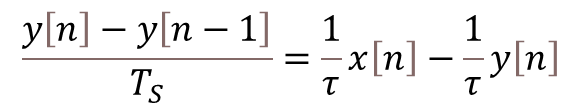
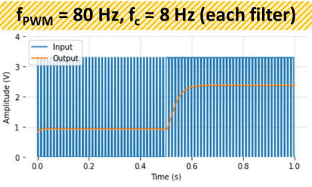
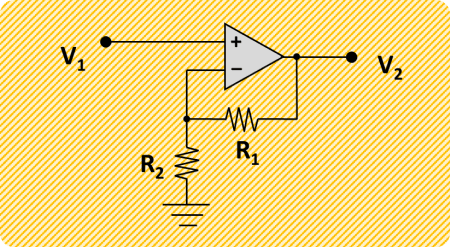
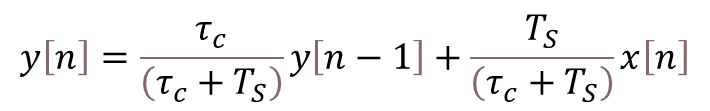
As I mentioned earlier in this post, the derivative term of the PID is quite sensitive to noise in the calculated error signal, which primarily comes from the transducers used to measure the plant output. One way to help mitigate this effect is the addition of a low-pass filter to the output of the derivative term inside the controller. Let’s use my favorite first-order digital filter, given by the difference equation below, whereis the derivative term output andis the corresponding filtered output signal.

PID Python Class

Finally, it’s time to put it all together inside a Python class. If you go through the code below, you’ll be able to identify all the components that were discussed in the previous three sections. The PID class should be instantiated before entering the execution loop, while the control method is called every time step inside the execution loop. In my next post we will use this class to control the speed of a small DC motor.

class PID:
    def __init__(self, Ts, kp, ki, kd, umax=1, umin=-1, tau=0):
        #
        self._Ts = Ts  # Sampling period (s)
        self._kp = kp  # Proportional gain
        self._ki = ki  # Integral gain
        self._kd = kd  # Derivative gain
        self._umax = umax  # Upper output saturation limit
        self._umin = umin  # Lower output saturation limit
        self._tau = tau  # Derivative term filter time constant (s)
        #
        self._eprev = [0, 0]  # Previous errors e[n-1], e[n-2]
        self._uprev = 0  # Previous controller output u[n-1]
        self._udfiltprev = 0  # Previous derivative term filtered value

    def control(self, ysp, y, uff=0):
        #
        # Calculating error e[n]
        e = ysp - y
        # Calculating proportional term
        up = self._kp * (e - self._eprev[0])
        # Calculating integral term (with anti-windup)
        ui = self._ki*self._Ts * e
        if (self._uprev+uff >= self._umax) or (self._uprev+uff <= self._umin):
            ui = 0
        # Calculating derivative term
        ud = self._kd/self._Ts * (e - 2*self._eprev[0] + self._eprev[1])
        # Filtering derivative term
        udfilt = (
            self._tau/(self._tau+self._Ts)*self._udfiltprev +
            self._Ts/(self._tau+self._Ts)*ud
        )
        # Calculating PID controller output u[n]
        u = self._uprev + up + ui + udfilt + uff
        # Updating previous time step errors e[n-1], e[n-2]
        self._eprev[1] = self._eprev[0]
        self._eprev[0] = e
        # Updating previous time step output value u[n-1]
        self._uprev = u - uff
        # Updating previous time step derivative term filtered value
        self._udfiltprev = udfilt
        # Limiting output (just to be safe)
        if u < self._umin:
            u = self._umin
        elif u > self._umax:
            u = self._umax
        # Returning controller output at current time step
        return u
Digital Filtering

Digital Filtering

After a continuous signal goes through an analog-to-digital conversion, additional digital filtering can be applied to improve the signal quality. Whether the signal is being used in a real-time application or has been collected for a later analysis, implementing a digital filter via software is quite straightforward. We already saw them being casually used in some of my previous posts, such as MCP3008 with Raspberry Pi. Now, let’s go over these types of filters in more detail. For the examples, we will be using the signal processing functions from the the SciPy Python package.

One of the drawbacks of digital filtering (or analog filtering, for that matter) is the introduction of a phase delay in the filtered signal.

The plots on the left illustrate what an actual filtered signal and its phase lag would look like (top), in contrast with an ideal filtered signal with no lag (bottom). While the ideal situation cannot be achieved with real-time signal processing, it can be achieved when processing signals that are already sampled and stored as a discrete sequence of numerical values.

Since the sequence from start to finish is available, the idea is to filter it once (causing a phase shift) and then filter the resulting sequence backwards (causing a phase shift again). Since the filtering is done both forward and backwards, the phase shifts cancel each other, thus resulting in a zero-phase filtered signal!

To see how it’s done, check out the filtfilt function and the very good application examples on the SciPy documentation. You can also go for the code used to generate the plots above on my GitHub page. I should note that I use filtfilt all the time in my signal processing endeavors. There’s a lot of information that can be extracted from a signal after you clean it up a little bit. If the time alignment between events is critical, avoiding a phase shift is the way to go.

Before we get into the real-time application of digital filters, let’s talk briefly about how they’re implemented. I’ll focus on filters that can be described as the difference equation below:

whereis the input sequence (raw signal) andis the output sequence (filtered signal). Before you abandon this webpage, let me rewrite the equation so we can start bringing it to a more applicable form. Since the idea is to find the outputas a function of its previous values and the input, we can go with:

It’s common to normalize the coefficients so . Also, for simplicity, consider a first order filter which, in terms of difference equations, only depends on the values of the current and last time steps, or and . Thus:

So, to build a first-order low-pass digital filter, all we need to do is determine the coefficients , and. Luckily for us, the SciPy MATLAB-Style filter design functions return those coefficients, reducing our task to just the implementation of the filter using Python. Before we go over a couple of code examples, let’s examine a first-order filter that I use quite a bit.

Backward Difference Digital Filter

Going from the continuous domain to the discrete domain involves a transformation where we approximate a continuous variable by its discrete equivalent. I will start with a first-order low-pass filter, by analyzing its continuous behavior, more specifically the response to a unit step input.

The continuous system response to the constant input is given by , whereis the response time of the filter and is related to the filter cutoff frequencyby:

The response time of the filter is the time it takes for the output to reach approximately 63 % of the final value. In the case of the graph above, the response time is 0.1 seconds. If you’re wondering where that comes from, just calculate the system response using .

The differential equation that corresponds to the first order continuous system in question is:

And here is where our discrete approximation ofusing backward difference (with sampling period) comes into play:

By also transformingandinto their discrete counterpartsand, we can arrive to the difference equation below, which represents the first-order low-pass digital filter, where we used backward difference to approximate. Remember that and are the discrete current and previous time steps.

Finally, solving forgives us an equation very similar to the one we saw at the end of the previous section. Note that the coefficients andare a function of the sampling rate and the filter response time (in this particular case).

What I like about this filter implementation is that it’s fairly straightforward to see that the outputis a weighed average of its previous valueand the current input value. Furthermore, the smaller the response time (), the faster the filter is (higher cutoff frequency) and the more it follows the input value. Conversely, the slower the filter (), the more the output takes into account the previous value.

The Python code below shows how to implement this filter by placing it inside an execution loop and running a step input excitation through it. It will produce the plot shown at the beginning of this section. I invite you to experiment with different response times (cutoff frequencies) and sampling periods.

import numpy as np
import matplotlib.pyplot as plt

# Creating time array for "continuous" signal
tstop = 1  # Signal duration (s)
Ts0 = 0.001  # "Continuous" time step (s)
Ts = 0.02  # Sampling period (s)
t = np.arange(0, tstop+Ts0, Ts0)

# First order continuous system response to unit step input
tau = 0.1  # Response time (s)
y = 1 - np.exp(-t/tau)  # y(t)

# Preallocating signal arrays for digital filter
tf = []
yf = []

# Initializing previous and current values
xcurr = 1  # x[n] (step input)
yfprev = 0  # y[n-1]
yfcurr = 0  # y[n]

# Executing DAQ loop
tprev = 0
tcurr = 0
while tcurr <= tstop:
    # Doing filter computations every `Ts` seconds
    if (np.floor(tcurr/Ts) - np.floor(tprev/Ts)) == 1:
        yfcurr = tau/(tau+Ts)*yfprev + Ts/(tau+Ts)*xcurr
        yfprev = yfcurr
    # Updating output arrays
    tf.append(tcurr)
    yf.append(yfcurr)
    # Updating previous and current "continuous" time steps
    tprev = tcurr
    tcurr += Ts0

# Creating Matplotlib figure
fig = plt.figure(
    figsize=(6.3, 2.8),
    facecolor='#f8f8f8',
    tight_layout=True)
# Adding and configuring axes
ax = fig.add_subplot(
    xlim=(0, max(t)),
    xlabel='Time (s)',
    ylabel='Output ( - )',
    )
ax.grid(linestyle=':')
# Plotting signals
ax.plot(t, y, linewidth=1.5, label='Continuous', color='#1f77b4')
ax.plot(tf, yf, linewidth=1.5, label='Discrete', color='#ff7f0e')
ax.legend(loc='lower right')

SciPy Butterworth Digital Filter

The non-functional code snippet below shows how to import the SciPy signal processing module an use it to create a first-order digital Butterworth filter. Note that the implementation of the filter in the DAQ execution loop is very similar to what was done in the example code above. In this particular case however, you should be able to immediately identify the difference equation for the filter

where the arrays containing the coefficients , and, are the output of the SciPy function signal.butter for the corresponding cutoff frequency and discrete sampling period.

# Importing SciPy module
from scipy import signal

#
# Doing other initialization
#

# Discrete signal parameters
tsample = 0.01  # Sampling period for code execution (s)
fs = 1/tsample  # Sampling frequency (Hz)

# Finding a, b coefficients for digital butterworth filter
fc = 10  # Low-pass cutoff frequency (Hz)
b, a = signal.butter(1, fc, fs=fs)

# Preallocating variables
xcurr = 0  # x[n]
ycurr = 0  # y[n]
xprev = 0  # x[n-1]
yprev = 0  # y[n-1]

tprev = 0
tcurr = 0
# Executing DAQ loop
while tcurr <= tstop:
    # Doing I/O tasks every `tsample` seconds
    if (np.floor(tcurr/tsample) - np.floor(tprev/tsample)) == 1:
        # Simulating DAQ device signal acquisition
        xcurr = mydaq.value
        # Filtering signal (digital butterworth filter)
        ycurr = -a[1]*yprev + b[0]*xcurr + b[1]*xprev
        yprev = ycurr
    # Updating previous values
    xprev = xcurr
    tprev = tcurr
    # Incrementing time step
    tcurr += Ts0

Finally, as I mentioned at the top, you can implement higher order or different types of filters. Take a look at the signal.iirnotch filter, which is a very useful design that removes specific frequencies from the original signal, such as the good old 60 Hz electric grid one.

Digital-to-Analog Conversion

Digital-to-Analog Conversion

As the counterpart of analog-to-digital conversion, DAC will take a digital signal and convert it to an analog one. Paraphrasing what I mentioned in previous posts, ADC and DAC walk hand-in-hand bridging the gap between the continuous and discrete domains that modern machines and devices have to deal with.

Even though there are several types of DACs, I will talk about the PWM-based one, where a reference input voltage is switched (in the form of a digital train of pulses) into a low-pass analog filter, producing an analog output. Before we get there, let’s first talk about Pulse Width Modulation, a very clever way to go from the discrete to the continuous domain, invented in the mid-seventies. A PWM signal has two main characteristics: its frequency and its duty cycle.

The figure illustrates the frequency and the concept of duty cycle for a 10 Hz PWM signal. In this case, the period of the PWM is 1/fPWM = 0.1 s. The chosen duty cycle is 25 %, which corresponds to the time the output is “on” (0.025 s). During the remainder of the duration of the PWM period (0.075 s) the output is “off”. As a matter of fact, it’s the modulation of the duty cycle that will control the output level of the DAC system.

Since it’s either fully “on” or fully “off”, the PWM signal is fundamentally a digital one. It’s the frequency and duty cycle of that “on-off” train of pulses, coupled with the response of the sub-system it’s interacting with, that will result in an analog behavior of the output of the overall system, in our case the digital-to-analog converter.

As a side note, the Python code used to generate the graphs in this post can be found on my GitHub page. Make sure to check it out and experiment with the DAC parameters.

The simplest DAC implementation is shown on the left. It consists of a low-pass first-order passive RC filter connected to the PWM output signal Vref. Typically, for a TTL circuit, the voltage can be either 0 (low) or 3.3V (high).

The cutoff frequency (rad/s) of the filter is fc = 1/(RC). Along with the PWM frequency, it can be used to obtain the desired behavior of this simple DAC.

Output Ripple

The PWM signal can be thought as a sequence of low-to-high and high-to-low step inputs into the RC filter. Even with a constantly switching input, this first order system will eventually produce a near constant output. The figures below show the effect of the RC filter cutoff frequency fc as well as the PWM frequency fPWM on the amplitude of the output ripple.

As it can be observed in the plots above, the output voltage will converge to (duty cycle) x Vref , which for the duty cycle of 25 % (used in the example) produces an output of 0.825 V when Vref = 3.3 V. Also, reducing the filter cutoff frequency or increasing the PWM frequency are both effective in reducing the output signal ripple. While having a slow RC filter can greatly reduce the ripple, that will negatively affect the DAC response time when it’s subject to a change in the desired output value.

DAC Step Response

In the case of our DAC, its response time is essentially the response time of the RC filter, i.e. 1/fc = RC (with fc in rad/s). Leaving the details for a future post on analog and digital filtering, for the first order system under consideration, the response time can be defined as the time it takes for the output to reach about 63 % of its final (steady-state) value, after a step input is applied.

The next figure shows how an appropriate combination of a higher PWM frequency and a higher filter cutoff frequency can produce a faster response time, while maintaining roughly the same amplitude of the DAC output ripple. For our example, the response time based on the RC value goes from 0.16 s down to 0.04 s.

Cascaded Filters

The output ripple can be further improved by cascading two first-order RC filters, as shown below. The newly formed second-order filter will have twice the attenuation (dB/decade) above the cutoff frequency. It’s an easy-to-do improvement which is often adopted.

Practical Considerations

Just like its ADC counterpart, DACs also have an inherent quantization in the signal. The digital PWM, generated from the microprocessor clock, has a finite resolution (duty cycle levels) given by the number of bits of the PWM. Typical resolutions range from 8 to 12 bits.

Actual PWM frequencies for DAC devices are much higher than the ones used in the examples above, which were chosen mainly to illustrate the concepts. For applications involving testing of physical systems or automation, frequencies between 500 and 2000 Hz are reasonable. In audio applications, several times the highest frequency of the audible range (20 kHz) seems to be the case. That is, 100 to 200 kHz. However, just as we observed when using higher order filtering, there’s wiggle room to reduce these numbers while still having a good compromise between response time and ripple.

It’s important to make a distinction at this point: if the PWM is used to drive a DC motor directly (or with some power amplification), the motor itself will behave approximately as a first order system. Hence, there’s no need for the RC filter. In this type of application, PWM frequencies of 100 to 200 Hz are just fine.

Amplification of the DAC output beyond the typical 3.3V Vref, can be achieved by using an Op Amp (Operational Amplifier). For a simple non-inverting amplifier, the output voltage is given by:

V2 = V1(1+R1/R2)

By choosing R1 = R2 = 10 kOhm, we can double the output to accommodate a more typical 0 to 5V requirement.

In my next post, we will explore the implementation of a DAC using a Raspberry Pi and a few resistors and capacitors. The Pi has hardware enabled PWM on two of its GPIO pins, which can reach frequencies in the kHz range! That should be an interesting project.

MCP3008 with Raspberry Pi

MCP3008 with Raspberry Pi

Since the Raspberry Pi is fundamentally a digital device, any I/O that is done through it’s GPIO pins will happen through high (one) and low (zero) states. When it comes to input signals that are analog, most likely from a transducer, they need to be converted to the digital domain so the Raspberry Pi can understand them. The MCP3008 is a 10-bit 8-channel analog-to-digital converter chip that has a very straightforward API implementation in GPIO Zero. The MCP3008 device uses an SPI (Serial Peripheral Interface) communication protocol that is fully taken care by the API.

SPI requires four pins for the communication:

  • A “SCLK” pin which provides the clock (pulse train) for the communication.
  • A “MOSI” pin (Master Out, Slave In) which the Pi uses to send information to the device.
  • A “MISO” pin (Master In, Slave Out) which the Pi uses to receive information from the device.
  • A “CEX” pin which is used to start and end the communication with the device, usually for one data sample at a time. Because the Raspberry Pi can have more than one device sharing the same SCLK, MOSI, and MISO pins, the CE0 or CE1 pin will indicate which device to use.

Additionally, the MCP3008 requires two separate voltage inputs ranging from 2.7 to 5.5V. The supply voltage at 5V allows for a higher data sampling rate of 200 kSamples/s (which should be plenty for the Raspberry Pi). A reference voltage of 3.3V improves the absolute resolution to about 3 mV instead of 5 mV since, for a 10-bit device, 1LSB = VREF/1024. However, the choice of VREF also has to satisfy the analog input range requirement of the transducer. If the input is higher that 5V, a resistive voltage divider can be used. Finally, in the case of a Raspberry Pi, both the digital and analog grounds on the device can share the same GND pin.

Important! You must enable the SPI for the MCP3008 communication to work. To do so, go to the Raspberry Pi Configuration menu and select Enable for the SPI in the Interfaces tab.

Hardware vs. Software SPI implementation

The Raspberry Pi has both a hardware and a software implementation of the SPI protocol. It is worth investigating what kind of sampling rates can be achieved with those two types.

The figure on the left shows a comparison between software and hardware implementation results of the sampling period per channel as a function of the number of analog inputs. The code used to collect the data, as well as GPIO pin configurations, can be found on my GitHub page.

For each point on the graph, data was sampled as fast as possible, i.e., with no time step clock, where the only I/O occurring in the execution loop was reading the MCP3008 output. Computational time storing the data in an array was negligible. Not surprisingly, the sampling period increases linearly with the number of input channels and, on my Raspberry Pi 4B, the hardware implementation is in average 3.6 times faster than the software one.

The hardware sampling rate is approximately 6.25 kSamples/s and the software one is approximately 1.72 kSamples/s. Note that it’s common to use Samples (or kSamples) per second for a DAQ device, where the number usually gives the maximum throughput of the device. For example, 5 channels with the hardware implementation still gives 6.25 kSamples/s. However the rate is 1.25 kSamples/s per channel.

Still on the 5 channels example, you can very likely get away without an anti-aliasing filter. Noise above 625 Hz (half of the 1250 Hz sampling rate) should have negligible amplitude and shouldn’t show up as an alias in the actual signal. That doesn’t mean that the analog signal being collected with the MCP3008 doesn’t have (relatively) low frequency noise, which in turn can be filtered using a digital low-pass filter in the DAQ software.

Example with a Potentiometer

A potentiometer is basically a variable resistive voltage divider that will output a voltage between a high and a low voltage value, in our case VREF and GND. Because potentiometers convert a linear or angular position input to a voltage output, they do fall into the transducer category.

In this example, the analog output of the potentiometer will be sampled by the DAQ software. To add a bit of visual excitement, the sampled voltage will be used to change the PWM output that controls the intensity of the LED.

The wires on the right hand side of the figure are all connected to the appropriate pins on the Raspberry Pi. Since hardware SPI will be used:

  • SCLK = GPIO11
  • MISO = GPIO9
  • MOSI = GPIO10
  • CEO = GPIO8

PWM is connected to GPIO16. Note that the LED requires a series resistor, where R can be anywhere between 300 to 1000 Ohm.

Also, pay attention to the semi-circular notch on the MCP3008 chip, so it can be inserted with the right orientation into the breadboard.

The Python code for the example is shown below, where there are a few things worth mentioning:

  • The sampling period is 0.02 s, which gives a sampling rate of 50 Samples/s. That is far below the limit for the hardware SPI implementation (6.25 kSamples/s) and even the software one (1.72 kSamples/s).
  • The execution loop concept with a time step clock is used to ensure a fairly accurate sampling period. Both I/O and computation tasks are performed within a time step with plenty of time to spare.
  • Due to the noise in the analog signal, most likely due to the questionable quality of the potentiometer, a digital low-pass filter is implemented in the code. The cutoff frequency of 2 Hz can be modified for some extra exploration of its effect.
  • For the plotting of the sampled signal to work, a module named utils.py has to be accessible for importing as discussed in my previous post A useful Python plotting module.
import time
import numpy as np
from utils import plot_line
from gpiozero import PWMOutputDevice, MCP3008

# Creating LED PWM object
led = PWMOutputDevice(16)
# Creating ADC channel object
pot = MCP3008(channel=0, clock_pin=11, mosi_pin=10, miso_pin=9, select_pin=8)
# Assining some parameters
tsample = 0.02  # Sampling period for code execution (s)
tstop = 10  # Total execution time (s)
vref = 3.3  # Reference voltage for MCP3008
# Preallocating output arrays for plotting
t = []  # Time (s)
v = []  # Potentiometer voltage output value (V)
vfilt = []  # Fitlered voltage output value (V)
# First order digital low-pass filter parameters
fc = 2  # Filter cutoff frequency (Hz)
wc = 2*np.pi*fc  # Cutoff frequency (rad/s)
tau = 1/wc  # Filter time constant (s)
c0 = tsample/(tsample+tau)  # Digital filter coefficient
c1 = tau/(tsample+tau)  # Digital filter coefficient
# Initializing filter previous value
valueprev = pot.value
time.sleep(tsample)
# Initializing variables and starting main clock
tprev = 0
tcurr = 0
tstart = time.perf_counter()

# Execution loop
print('Running code for', tstop, 'seconds ...')
while tcurr <= tstop:
    # Getting current time (s)
    tcurr = time.perf_counter() - tstart
    # Doing I/O and computations every `tsample` seconds
    if (np.floor(tcurr/tsample) - np.floor(tprev/tsample)) == 1:
        # Getting potentiometer normalized voltage output
        valuecurr = pot.value
        # Filtering value
        valuefilt = c0*valuecurr + c1*valueprev
        # Calculating current raw and filtered voltage
        vcurr = vref*valuecurr
        vcurrfilt = vref*valuefilt
        # Updating LED PWM output
        led.value = valuefilt
        # Updating output arrays
        t.append(tcurr)
        v.append(vcurr)
        vfilt.append(vcurrfilt)
        # Updating previous filtered value
        valueprev = valuefilt
    # Updating previous time value
    tprev = tcurr

print('Done.')
# Releasing pins
pot.close()
led.close()
# Plotting results
plot_line([t]*2, [v, vfilt], yname='Pot Output (V)', legend=['Raw', 'Filtered'])
plot_line([t[1::]], [1000*np.diff(t)], yname='Sampling Period (ms)')

The graphs below show the results of one run on my Raspberry Pi 4B. Observe how the low-pass filter removes the noise from the raw signal as I twirl around the potentiometer knob. That of course comes with a price: the filtered signal now lags the original signal. In DAQ applications where the signal doesn’t need to be filtered in real-time, there are “zero-lag” filtering techniques that can be applied after the signal was acquired. Also note the consistent sampling time step of 20 ms.

A note on Quantization

What would happen if I never touched the potentiometer during the program execution, leaving its output at a constant value? The result is shown in the next graph, where the quantization effect is quite clear on the (very low amplitude) signal noise riding on top of the output voltage. The discrete nature of the output can now be observed, and the values are exactly VREF/210 = 3.3/1024 = 0.0032 V apart!

Analog-to-Digital Conversion

Analog-to-Digital Conversion

Also known as ADC, is the process of converting a physical quantity, usually represented by a voltage at this point, to a set of bits that’s more suitable for a computer to digest. Bearing in mind that the world we live in is analog in nature and the computers we use to interact with it are digital, going from the continuous domain to the discrete domain is an integral part of most machines and devices out there.

Back in the day, when micro-processors and computers weren’t around or were still in their infancy, many systems would function entirely in the analog domain. Take for instance an old record player. From the needle running in the record tracks (a continuous profile of peaks and valleys) to the sound coming out of the speakers, the entire sequence of changes in physical quantities occurred in the analog domain. Nowadays, still on the same example, music is stored as digital content and only converted back to an analog signal when it’s time to make it to the speakers, so we can listen to it with our good old analog ears. This last process of going back from the discrete to the analog domain is handled through a digital-to-analog conversion (DAC) and will be a topic of another post. The entire process can be illustrated with the diagram below.

As I alluded to at the very top, a sensor (or more specifically a transducer) will convert the measured physical quantity to an electrical signal, and ultimately a voltage. The next step in the process is the signal conditioning where some sort of filtering will be applied to the measured voltage. Not only to avoid aliasing, which we will discuss later on, but some times to accomplish other goals, like for example remove a DC component or a very slow drift in the signal.

The next block is the analog-to-digital conversion (ADC), which has mainly two tasks to it: sampling and quantization. Once they are performed, the continuous signal will be broken down into packets of bits that the computer can now handle. We will see that the signal is not only discrete in time but also each sample can only have a finite number of values.

At the bottom half of the diagram is the flip side of the coin: the digital-to-analog (DAC) conversion, an eventual power amplification and, generally speaking, the electro-mechanical actuators.

You should also note that if we are talking about data acquisition only, the focus is the top half of the diagram. If automation is the case, then the entire diagram is in scope.

Sampling

A physical system changes its states continuously over time and it would be impractical to collect continuous data to be used by an inherently discrete system such as the computer. Using the music example, and going back several decades, data would be collected and recorded on magnetic tapes so it could be later edited, mixed, and reproduced. With the computer entering the landscape, those analog systems had their days numbered.

The sampling process occurs in an integrated circuit (IC), where an electronic switch will bring a sample of the signal into the AD converter at a fixed sampling period.

The figure on the right shows 2 seconds of an arbitrary continuous signal sampled at 0.1 seconds (or 10 Hz). The first thing to notice is that we can now store 20 data points instead of an impractical infinite number of continuous points.

There are other considerations that dictate the sampling period (or frequency) than just the amount of data that can be manipulated. The main one is the frequency content of the signal. In other words, how “fast” does the signal change over time. For good signal reconstruction in the time domain, a sampling rate of 10 to 20 times the frequency content of the signal should be used. Most importantly, it must never be below 2 times the highest frequency component of the measured signal. Otherwise, aliasing will potentially occur to the sampled data.

As a quick note, all the plots used in this post were generated using Python and the Matplotlib package. You can get the code on my GitHub page.

Nyquist Theorem and Aliasing

According to the Nyquist sampling theorem, the sampling rate should be at least two times the maximum frequency component of the measured signal. The figure below shows a 20 Hz sinusoidal signal sampled at 21 Hz. Any sampling rate below 40 Hz will result in an alias of the original signal. In this case a new 1 Hz sinusoidal wave will show up.

The frequency of the aliased signals (yes, there’s more than one alias) is not exactly intuitive, as it appears to be in the previous figure. The same original 20 Hz signal sampled at 7 Hz would also produce a 1 Hz aliased signal! Check out the Python code on my GitHub page for a couple of formulas and to explore different sampling rates.

In practical terms, it is hard to guarantee that the signal being sampled won’t contain stray frequencies above the Nyquist frequency. The best way to avoid aliasing is to use an analog low-pass filter before the signal is sampled. Even a simple passive RC filter should suffice, provided a reasonable frequency transition band to accommodate for the poor filter attenuation right above its cut-off frequency.

Back to the music example, audio is usually sampled at 44.1 kHz. Since the human ear can respond to frequencies up to about 20 kHz, sound should be sampled at least at 40 kHz. 44.1 kHz gives a Nyquist frequency of 22.05 kHz and therefore a transition band of 2.05 kHz for a filter with a cut-off frequency of 20 kHz. However, it’s not uncommon to record audio at 48 kHz (or even 96 kHz). The former gives a Nyquist frequency of 24 kHz and therefore a wider 4 kHz transition band for a low-pass filter to attenuate the signal above it’s cut-off frequency of 20 kHz.

For the classically inclined, how does 48 kHz compare with the frequency contents of the music that’s being recorded? A soprano can hit C6 (1046.5 Hz), a violin A7 (3520 Hz), and a piano C8 (4186.01 Hz). Those frequencies are well bellow the Nyquist frequency of 24 kHz and even 10 times (or more) lower than the 48 kHz sampling frequency, allowing also for good signal reconstruction in the time domain.

Quantization

The second task in the AD processing is the quantization of the sampled values. Even though your computer can deal with floating numbers (they’re still a bunch of bits in disguise), the ADC device still ships out a packet of bits for every analog sample. The analog value will be discretized based on a reference voltage and the number of bits used for the quantization.

The ideal transfer function (TF) between the analog input voltage and the digital output code is a straight line where for every possible input there’s a unique output. In other words, the ideal ADC has an infinite resolution. Because the output of the conversion is a digital value, the transfer function of a perfect ADC is in fact a staircase function where each step is 1 LSB (Least Significant Bit).

As shown in the figure, let’s consider the case with a reference voltage VREF = 2 V and a resolution of 3 bits. The step size (1 LSB) is 0.25 V, or in the general case VREF / 2n, where n is the number of bits of the ADC.

Any analog input within a step will be coded to the same digital output. For example, 0.625 to 0.875 V will be coded as 011 (or 3 in decimal representation). Using the reference voltage of 2 V, that would give us 3VREF / 8 = 0.75 V. Therefore, the quantization error goes from +0.125 V to -0.125 V. In other words +/- 0.5 LSB. This would be the case for the perfect ADC shown in the figure, more specifically a single-ended mode configuration with adjusted quantization. A good source explaining other configurations and also sources of errors that occur on an actual ADC can be found here. The full scale (FS in the figure) is VREF – 1LSB, which in the case of this example would be 1.75 V.

If a 4-bit converter is used, the quantization error for the same reference voltage drops to +/- 0.0625 V (still +/- 0.5 LSB) and the FS goes up to 1.875 V.

As we move up in bit resolution, the ADC output starts to approximate the ideal transfer function. In the case of a 10-bit ADC, the quantization error becomes +/- 0.5VREF/1024. Which in our case is approximately +/- 0.001 V, and in the general case +/- 0.05 % of the reference voltage. For a high accuracy 16-bit ADC, the error is approx. +/- 0.0008 % of the reference voltage.

Note that there are additional errors introduced in the quantization process due to offsets, non-linearities, and just noise in general in the electronic circuitry. A 12-bit converter will typically have +/- 0.13 % (instead of +/- 0.012 %) and a 16-bit a typical +/- 0.01%.

Practical Considerations

So, how high should you go with the sampling rate and number of quantization bits? How about the anti-aliasing filter? Keep in mind that faster, higher-resolution hardware comes with a steeper cost. And high sampling rates bring the burden of extra storage space and processing power.

If you are working with audio, definitely 48 kHz and 16-bit ADC for sound recording. 96 kHz (or even 172 kHz) and 24-bit if you’re a pro. And most definitely an anti-alias filter. By the way, the fact that 96 kHz is two times the 48 kHz base rate makes it very easy to down sample a recording for later reproduction: just throw away every other data point.

If you’re toying around with a Raspberry Pi, the sampling rate is the one that suits your needs. For slow changing temperatures 1 Hz is plenty. Pressures maybe 10 to 20 Hz. A 10-bit ADC MCP3008 chip is inexpensive and has plenty of resolution. An anti-aliasing filter is probably overkill. The higher frequency content of noise is also usually low amplitude and therefore shouldn’t affect you signal very much. However, it’s always a good idea to sample your data first at a higher frequency and inspect it as a function of time. Also, be careful with some typical electrical noise like the 60 Hz one caused by the AC outlet.

In a lab or instrumentation setting, 12 to 16-bit and an anti-aliasing filter, such as a simple passive RC one, should be considered. Again, try different sampling rates and filters. As I mentioned before, it’s always important to look at your data as a function of time first with as high as a sampling rate that can be run with the DAQ device at hand. Once you understand what the signal is all about, then a more conscious decision about the hardware requirements can be made.

Finally, just to have some fun with Python, below is the arbitrary signal of this post with two different sampling rates and resolutions. Observe the effects of both the sampling and the quantization on the original signal.

Execution Loops

Execution Loops

I like to divide execution loops into two main categories: Synchronous loops and Asynchronous loops. The first one does its tasks based on some sort of clock (or clocks) at a fixed sampling period (or periods). The second type performs its tasks based on events that are triggered by other parts of the program, or by external devices integrated into the program. If you’re using your mouse wheel to scroll down this web page, the wheel motion is an asynchronous event triggered by the mouse device that notifies the main application that something happened and that the wheel position data will be sent. The main application uses that data and then takes care of moving the page up.

Moving forward, let’s focus on synchronous execution loops. The most general code layout contains a group of tasks that are performed before the program starts the execution loop, the loop itself, and tasks that are performed after the loop finishes running. If DAQ devices are being used for instance, a typical task before starting the loop is to look for (and do some checks on) the DAQ device and then connect to it. After the loop finishes, properly disconnecting from the DAQ device is a typical task done at that time. Other tasks, such as loading and saving data, starting and stopping other processes or interfaces, also fall into the before and after categories.

The simplest possible code (shown below) only contains the execution loop and would run forever until the power is cut off or someone hits “CTRL” + “C” on the keyboard. While this is sometimes all that’s needed, I prefer to add some sort of exit condition.

import time
import datetime

# Doing tasks before entry condition
print('Running forever ...')
print('Interrupt or press "CTRL"+"C" to stop.')
# Running execution loop
while True:
    # Doing computations
    for i in range(100000):
        pass
    # Doing I/O tasks
    print('I/O at', datetime.datetime.now().time())
    # Pausing for 1 second
    time.sleep(1)
Running forever ...
Interrupt or press "CTRL"+"C" to stop.
I/O at 20:22:26.737740
I/O at 20:22:27.740305
I/O at 20:22:28.743494
I/O at 20:22:29.745530
I/O at 20:22:30.747698
I/O at 20:22:31.749704
I/O at 20:22:32.752015
I/O at 20:22:33.755986
I/O at 20:22:34.758986
I/O at 20:22:35.760987
I/O at 20:22:36.763165
I/O at 20:22:37.765439
I/O at 20:22:38.770925

You should first notice that on the output above on the right, the time step is slightly over 1 second. In this case, the longer the computations take, the farther away this number will be from 1 second. While you could account for the computational time and subtract it from the sleep duration, even the corrected value tends to drift over time, loosing it’s accuracy. Let’s improve that and add an exit condition by using a clock, as shown below. It could represent for how long a test needs to run. If the code is part of a GUI (Graphical User Interface), the entry and exit conditions could be just a start and a stop buttons.

import time
import datetime
import numpy as np

# Assigning time parameters
tsample = 1  # Data sampling period (s)
tstop = 100  # Test stop time (s)
# Initializing timers and starting main clock
tprev = 0  # Previous time step
tcurr = 0  # Current time step
tstart = time.time()
# Doing tasks before entry condition
print('Running for', tstop, 'seconds ...')
# Running execution loop
while tcurr <= tstop:
    # Updating previous time and getting current time (s)
    tprev = tcurr
    tcurr = time.time() - tstart
    # Doing computations
    for i in range(100000):
        pass
    # Doing I/O tasks every `tsample` seconds
    if (np.floor(tcurr/tsample) - np.floor(tprev/tsample)) == 1:
        print(
            'I/O at', datetime.datetime.now().time(),
            '(Elapsed time = {:0.3f} s)'.format(tcurr))
# Doing tasks after exit condition
print('Done.')
Running for 100 seconds ...
I/O at 20:27:43.673925 (Elapsed time = 1.001 s)
I/O at 20:27:44.671919 (Elapsed time = 2.000 s)
I/O at 20:27:45.675318 (Elapsed time = 3.002 s)
I/O at 20:27:46.675509 (Elapsed time = 4.003 s)
I/O at 20:27:47.674825 (Elapsed time = 5.002 s)
I/O at 20:27:48.673115 (Elapsed time = 6.000 s)
I/O at 20:27:49.673116 (Elapsed time = 7.000 s)
I/O at 20:27:50.674293 (Elapsed time = 8.001 s)
I/O at 20:27:51.675247 (Elapsed time = 9.002 s)
I/O at 20:27:52.674257 (Elapsed time = 10.001 s)
I/O at 20:27:53.675288 (Elapsed time = 11.002 s)
I/O at 20:27:54.674371 (Elapsed time = 12.001 s)
I/O at 20:27:55.673409 (Elapsed time = 13.000 s)
I/O at 20:27:56.675287 (Elapsed time = 14.002 s)
I/O at 20:27:57.674133 (Elapsed time = 15.001 s)
I/O at 20:27:58.674246 (Elapsed time = 16.001 s)
I/O at 20:27:59.673134 (Elapsed time = 17.000 s)
I/O at 20:28:00.675795 (Elapsed time = 18.003 s)
I/O at 20:28:01.674195 (Elapsed time = 19.001 s)
I/O at 20:28:02.674295 (Elapsed time = 20.001 s)
I/O at 20:28:03.675202 (Elapsed time = 21.002 s)
...
I/O at 20:29:19.674898 (Elapsed time = 97.002 s)
I/O at 20:29:20.674071 (Elapsed time = 98.001 s)
I/O at 20:29:21.672220 (Elapsed time = 99.000 s)
I/O at 20:29:22.675361 (Elapsed time = 100.003 s)
Done.

Observe that after adding the sampling clock condition, the elapsed time between steps is consistently 1 second (within a couple of milliseconds, as shown above on the right). Even if you were to run the code for an indefinite amount of time, the sampling period would stay consistent. As shown in the next piece of code, it is possible to add multiple clock conditions to the execution loop. For instance, one clock for data acquisition and one clock for data display.

import time
import datetime
import numpy as np

# Assigning time parameters
tsample = 0.2  # Data sampling period (s)
tdisp = 1  # Data display period (s)
tstop = 100  # Test stop time (s)
# Initializing timers and starting main clock
tprev = 0  # Previous time step
tcurr = 0  # Current time step
tstart = time.time()
# Doing tasks before entry condition
print('Running for', tstop, 'seconds ...')
# Running execution loop
while tcurr <= tstop:
    # Updating previous time and getting current time (s)
    tprev = tcurr
    tcurr = time.time() - tstart
    # Doing computations
    for i in range(100000):
        pass
    # Doing I/O tasks every `tsample` seconds
    if (np.floor(tcurr/tsample) - np.floor(tprev/tsample)) == 1:
        print(
            'I/O at', datetime.datetime.now().time(),
            '(Elapsed time = {:0.3f} s)'.format(tcurr))
    # Displaying data every `tdisp` seconds
    if (np.floor(tcurr/tdisp) - np.floor(tprev/tdisp)) == 1:
        print(
            'Displaying data',
            '(Elapsed time = {:0.3f} s)'.format(tcurr))
# Doing tasks after exit condition
print('Done.')
Running for 100 seconds ...
I/O at 10:18:01.743822 (Elapsed time = 0.201 s)
I/O at 10:18:01.944788 (Elapsed time = 0.402 s)
I/O at 10:18:02.144784 (Elapsed time = 0.603 s)
I/O at 10:18:02.347786 (Elapsed time = 0.803 s)
I/O at 10:18:02.545785 (Elapsed time = 1.002 s)
Displaying data (Elapsed time = 1.002 s)
I/O at 10:18:02.743788 (Elapsed time = 1.200 s)
I/O at 10:18:02.944790 (Elapsed time = 1.402 s)
I/O at 10:18:03.143787 (Elapsed time = 1.600 s)
I/O at 10:18:03.343785 (Elapsed time = 1.801 s)
I/O at 10:18:03.542788 (Elapsed time = 2.000 s)
Displaying data (Elapsed time = 2.000 s)
I/O at 10:18:03.742835 (Elapsed time = 2.200 s)
I/O at 10:18:03.943834 (Elapsed time = 2.402 s)
I/O at 10:18:04.144792 (Elapsed time = 2.602 s)
I/O at 10:18:04.343825 (Elapsed time = 2.801 s)
I/O at 10:18:04.542789 (Elapsed time = 3.000 s)
Displaying data (Elapsed time = 3.000 s)
I/O at 10:18:04.742791 (Elapsed time = 3.201 s)
I/O at 10:18:04.943792 (Elapsed time = 3.401 s)
I/O at 10:18:05.146791 (Elapsed time = 3.602 s)
I/O at 10:18:05.347791 (Elapsed time = 3.803 s)
I/O at 10:18:05.542792 (Elapsed time = 4.000 s)
Displaying data (Elapsed time = 4.000 s)
I/O at 10:18:05.745793 (Elapsed time = 4.203 s)
I/O at 10:18:05.945793 (Elapsed time = 4.402 s)
I/O at 10:18:06.142790 (Elapsed time = 4.600 s)
...
I/O at 10:19:41.143165 (Elapsed time = 99.600 s)
I/O at 10:19:41.342204 (Elapsed time = 99.800 s)
I/O at 10:19:41.544215 (Elapsed time = 100.001 s)
Displaying data (Elapsed time = 100.001 s)
Done.

Finally, depending on what you’re trying to do and how the code is laid out, CPU usage could become significant. Always keep an eye out for that. On a Windows platform, you could use the Task Manager.