Author: Eduardo Nigro

7-Segment LED Display with Raspberry Pi

7-Segment LED Display with Raspberry Pi

These types of LED displays are quite popular and can be used to add a visual output to a Raspberry Pi automation project. In this post, I will be talking about the KS0445 4-digit LED Display Module from keyestudio. While keyestudio kits are primarily designed to work with Arduino, they are perfectly suitable for Pi applications.

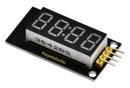
In theory, any LED 4-digit Display using a TM1637 chip can be used with the Python code that will be shown.

The first step is to install the TM1637 Python package containing the class that will simplify controlling the LED display quite a bit. As a side note, I strongly encourage installing VS Code on the Pi, so you can code like a pro.

Open a terminal window in VS Code and type:

pip install raspberrypi-tm1637

Once the installation is complete, you can wire the display as shown below and try the Python code that follows. It illustrates how straightforward it is to use some of the methods of the TM1637 class that come in the package.

# Importing modules and classes
import tm1637
import time
import numpy as np
from datetime import datetime
from gpiozero import CPUTemperature

# Creating 4-digit 7-segment display object
tm = tm1637.TM1637(clk=18, dio=17)  # Using GPIO pins 18 and 17
clear = [0, 0, 0, 0]  # Defining values used to clear the display

# Displaying a rolling string
tm.write(clear)
time.sleep(1)
s = 'This is pretty cool'
tm.scroll(s, delay=250)
time.sleep(2)

# Displaying CPU temperautre
tm.write(clear)
time.sleep(1)
cpu = CPUTemperature()
tm.temperature(int(np.round(cpu.temperature)))
time.sleep(2)

# Displaying current time
tm.write(clear)
time.sleep(1)
now = datetime.now()
hh = int(datetime.strftime(now,'%H'))
mm = int(datetime.strftime(now,'%M'))
tm.numbers(hh, mm, colon=True)
time.sleep(2)
tm.write(clear)

Raspberry Pi Stopwatch with LED Display

That was pretty much it for the LED display. However, let’s go for an Easter egg, where we implement a stopwatch that can be controlled by keyboard inputs. The main feature here is the use of the Python pynput package, which seamlessly enables non-blocking keyboard inputs. To get started, in a terminal window in VS Code, type:

pip install pynput

To make things more interesting, I created the class StopWatch with the following highlights:

  • First and foremost, could the entire code be written using a function (or a few functions) or even as a simple script? Yes, it could. However, using a class makes for code that is much more modular and expandable, and that can easily be integrated into other code.
  • At the center of the the StopWatch class is the execution loop method. For conciseness and readability, all other methods (with very descriptive names) are called from within this execution loop.
  • The beauty of using a class and therefore its methods is that the latter can be called from different points in the code, as it is the case of the start_watch() method, for example.
  • Finally, as the code is written as a class vs. functions, all the variables can be defined as class attributes. That really reduces complexity with input arguments, if functions were to be used instead.
# Importing modules and classes
import time
import tm1637
import numpy as np
from pynput import keyboard


class StopWatch:
    """
    The class to represent a digital stopwatch.

    **StopWatch** runs on a Raspberry PI and uses a 4-digit 7-segment display
    with a TM1637 control chip.

    The following keyboard keys are used:

        * ``'s'`` to start/stop the timer.
        * ``'r'`` to reset the timer.
        * ``'q'`` to quit the application.

    """
    def __init__(self):
        """
        Class constructor.

        """
        # Creating 4-digit 7-segment display object
        self.tm = tm1637.TM1637(clk=18, dio=17)  # Using GPIO pins 18 and 17
        self.tm.show('00 0')  # Initializing stopwatch display
        # Creating keyboard event listener object
        self.myevent = keyboard.Events()
        self.myevent.start()
        # Defining time control variables (in seconds)
        self.treset = 60  # Time at which timer resets
        self.ts = 0.02  # Execution loop time step
        self.tdisp = 0.1  # Display update period
        self.tstart = 0  # Start time
        self.tstop = 0  # Stop time
        self.tcurr = 0  # Current time
        self.tprev = 0  # Previous time
        # Defining execution flow control flags
        self.run = False  # Timer run flag
        self.quit = False  # Application quit flag
        # Running execution loop
        self.runExecutionLoop()

    def runExecutionLoop(self):
        """
        Run the execution loop for the stopwatch.

        """
        # Running until quit request is received
        while not self.quit:
            # Pausing to make CPU life easier
            time.sleep(self.ts)
            # Updating current time value
            self.update_time()
            # Handling keyboard events
            self.handle_event()
            # Checking if automatic reset time was reached
            if self.tcurr >= self.treset:
                self.stop_watch()
                self.reset_watch()
                self.start_watch()
            # Updating digital display
            self.update_display()
            # Stroing previous time step
            self.tprev = self.tcurr

    def handle_event(self):
        """
        Handle non-blocking keyboard inputs that control stopwatch.

        """
        # Getting keyboard event
        event = self.myevent.get(0.0)
        if event is not None:
            # Checking for timer start/stop
            if event.key == keyboard.KeyCode.from_char('s'):
                if type(event) == keyboard.Events.Release:
                    if not self.run:
                        self.run = True
                        self.start_watch()
                    elif self.run:
                        self.run = False
                        self.stop_watch()
            # Checking for timer reset
            elif event.key == keyboard.KeyCode.from_char('r'):
                if type(event) == keyboard.Events.Release:
                    if not self.run:
                        self.reset_watch()
                    elif self.run:
                        print('Stop watch before resetting.')
            # Checking for application quit
            elif event.key == keyboard.KeyCode.from_char('q'):
                self.quit = True
                self.tm.write([0, 0, 0, 0])
                print('Good bye.')

    def start_watch(self):
        """ Update start time. """
        self.tstart = time.perf_counter()

    def stop_watch(self):
        """ Update stop time. """
        self.tstop = self.tcurr

    def reset_watch(self):
        """ Reset timer. """
        self.tstop = 0
        self.tm.show('00 0')

    def update_time(self):
        """ Update timer value. """
        if self.run:
            self.tcurr = time.perf_counter() - self.tstart + self.tstop

    def update_display(self):
        """ Update digital display every 'tdisp' seconds. """
        if (np.floor(self.tcurr/self.tdisp) - np.floor(self.tprev/self.tdisp)) == 1:
            # Creating timer display string parts (seconds, tenths of a second)
            if int(self.tcurr) < 10:
                tsec = '0' + str(int(self.tcurr))
            else:
                tsec = str(int(self.tcurr))
            ttenth = str(int(np.round(10*(self.tcurr-int(self.tcurr)))))
            # Showing string on digital display
            self.tm.show(tsec + ' ' + ttenth)


# Running instance of StopWatch class
if __name__ == "__main__":
    StopWatch()
DC Motor Characterization (2 of 2)

DC Motor Characterization (2 of 2)

Picking it up from where we stopped in the previous post, let’s see how we can determine the effective moment of inertia, the effective damping and the torque constant for the reduced order model shown in the diagram.

Before we start, it’s a good idea to revisit a typical set of torque/speed curves for a DC motor. They will come in handy to better understand the parameter determination (identification) tests that are explained further down the post.

The graph shows torque/speed curves at constant input voltages for a DC motor, for arbitrarily chosen levels of 40, 60, 80 and 100%.

The torque values on the zero-speed y-axis represent the motor stall torque at different input voltages. Conversely, the speed values on the zero-torque x-axis represent the unloaded maximum motor speed, also at different input voltages.

These two special sets of data points will be used to determineandrespectively.

This time around, I’ll use a LEGO Mindstorms EV3 large motor. The basic reason behind such hardware choice is the easiness to build different test fixtures based on the parameter that’s being identified.

Determination of DC Motor Torque Constant

The torque constantcan be determined through a series of torque stall tests with varying motor input levels. The images below show the LEGO fixture that was built to accomplish the task.

The fixture design allows for the motor angular motion to be converted to a linear motion through the pulley system and the Nylon line. Therefore, the torque can be calculated from the measured linear force using the spring gauge.

Since the radius of the large pulley is known, the measured force in N can be converted to a measured torque in N.m.

The low budget gauge accuracy was verified with known masses and proved to be meet the standards of this blog. As a side note, calibration/verification of your measurement gauges should always be a part of any experimental testing!

Because of the nature of the force gauge, where the measurement readings had to be done visually by myself, it wasn’t possible to automate this test. Nonetheless, I used the pyev3 package to create a motor object and interactively set output levels.

It should be noted that the motor input can range between -100 and 100 %. The values are likely PWM duty cycle and seem to have a linear relationship with armature voltage (to which I don’t have access through the EV3 brick).

Finally, the mass of the spring gauge was taking into account when calculating the torque values.

The stall torque was measured for 4 large EV3 motors, where each point on the plot is the average of three torque values calculated from the corresponding force reading.

Four input levels were used, i.e., 40, 60, 80, and 100%. The dashed lines were fitted to the data points for each motor. Now, if we remember from the first test of the previous post that:

Then the slope of each line represents the torque constant in N.m/%. The average value is:

Determination of DC Motor Damping

Similarly to the torque constant determination, four large EV3 motors were used to generate the damping data. This time around however, because no torque load is applied to the motors, no fixture was required for the testing other than my hand holding the motor.

The plot shows the results for the zero-load tests, where each point is the average of three measurements for a given motor. The same input levels of the previous section were used.

If we reference back to the second test of the DC Motor Characterization (1 of 2) post, where:

The slope of the fitted dashed lines represents the speed constant in rad/s/%. The average value is:

Since we already know the value of the torque constant, the damping constant can then be calculated, leading to:

The Python code used to generate the plots and data fits above, as well as the automated test for the determination of the motor speed constant, can be found here.

Determination of DC Motor Inertia

The final parameter to be identified is the effective moment of inertia. As the name suggests, it accounts for the rotor inertia and any rotating masses attached to the output shaft. In the particular case of the EV3 motor, there’s a gearbox between the rotor and the output shaft. Therefore the moment of inertia of all the gears and the effect of the gear ratios will be accounted for, once we determine the effective moment of inertiareduced to the output shaft.

The moment of inertia will be estimated using the third test from the previous post as illustrated on the plot to the left. The idea is to determine the time constantof the approximated first order system and use

to determine since is already known.is the time to reach 63.2% of the steady-state speed value.

Some signal processing was used, as suggested in the graph above. A zero-shift low-pass filter was applied to the motor angular speed signal and thenwas calculated as the median value of the last 0.5 seconds of the signal. With the steady-state speed value in hands, can be easily determined and therefore .

Four different motors were tested at four input levels (40, 60, 80, and 100%), where five measurements were taken at each level. With a median time constantof 0.076 s, and using the the formula above with the already determined , The effective moment of inertia at the motor shaft output is:

Note that the effective moment of inertia is a fairly large number for such a small motor. Remember however that the moment of inertia at the shaft output is proportional to the squared value of the gear ratio. Which means, for our particular LEGO motor, if the gear ratio is for example 1:30, the rotor moment of inertia is 900 times smaller that the value at the gearbox output!

More on Effective Moment of Inertia

Let’s explore what happens if we attach an additional rotating mass to the shaft output, thus modifying the effective moment of inertia. One would expect the response time constant to increase as the rotating inertia increases.

To that end, the original test fixture was modified to accommodate two balanced counter weights. Such setup creates a zero load torque while allowing for different load inertias (by changing the mass of the counter weights).

Just for the sake of this exercise, let’s call the original effective moment of inertia of the LEGO large motor at the output shaft asand the additional inertia due to the counter-weights as . Note that

whereis the total mass of the counter-weights andis the radius of the pulley. The moment of inertia of the pulley is negligible when compared to that of the counter-weights.

Two sets of weights were used, i.e., 0.149 and 0.249 kg with a corresponding moment of inertia of 0.00023 and 0.00045 kg.m2 (the pulley radius is 39.25 mm). Using the formula below with all the known quantities allows us to calculate the time constant of the system with motor plus counter-weights.

In our case, the calculated values ofare 0.086 and 0.098 s. Running the test shown on the left, with four different motors and four different output levels, in fact produced measured values within +/- 3% of the corresponding calculated ones!

DC Motor Model Confirmation

It’s always a good idea to check whether the motor characterization parameters can be used to build a model that represents the actual system behavior. To do that, a set of counter-weight masses that haven’t been tested during the characterization was chosen, resulting in the following motor model.

Where the load torque due to the uneven counter-weight masses is 0.055 N.m and the effective inertia is 0.0014 + 0.00034 = 0.00174 kg.m2. The plot on the left shows good agreement between the actual LEGO fixture test results and the Simulink simulation of the reduced-order model above, for a 70% duty-cycle step input.

DC Motor Characterization (1 of 2)

DC Motor Characterization (1 of 2)

In this first of two posts, we’ll go over the simplifications of the equations that govern the dynamic behavior of a DC motor. By doing so, we should be able to use a non-intrusive and fairly straightforward approach to determine the parameters that characterize the motor from a control systems stand point.

While this might get a bit arid at times, I’ll try to keep it interesting by using some real motor parameters and Simulink to show the impact of the simplifications as we move towards our final dynamic system equation. Let’s start with the well known coupled differential equations (which are essentially a mathematical representation) for the electric motor:

Where (in SI units, for good measure):

By applying the Laplace transformation to the equations above and rearranging them in a way that they are solved for the angular velocity and current, we get:

and therefore

The rearranged equations can then be represented in the form of a block diagram, which will come in handy when we talk about the model simplification. Also, note the negative “feedback” nature of the back EMF term(which makes the rotor speed inherently stable to small disturbances in the load torque).

The DC motor has two time constants associated with its dynamic behavior. The electrical time constant(directly obtained from one of the first-order blocks in the diagram) and the mechanical time constant, which is not so intuitive and we’ll see later where it comes from.

Especially for smaller motors, the electrical time constant is substantially faster than the mechanical time constant. That is generally accompanied by, which means that the corresponding inductance term in the first-order block can be neglected. The block diagram of the resulting system is shown next.

It’s time to put some numbers into these two models and observe how they behave when simulated using Simulink. In order to do that, I found myself a motor data sheet for permanent magnet DC motors from Moog. These tend to be very high end components when compared to the DC motors I’ve been using in my previous posts. I.e. they are designed for a more professional application. Not for the “DIY-finite-budget-hobbyist”, like myself!

With that said, I chose the smallest and the largest motors from the catalog, whose parameters are summarized below:

C23-L33-W10C42-L90-W30
Lengthmm85229
Diametermm57102
Armature VoltageV (DC)1290
Rated CurrentA4.755
Rated Speedrad/s492159
Rated TorqueN.m0.052.26
Friction TorqueN.m0.020.17
Torque Constant ()N.m/A0.01870.5791
Back EMF Constant ()V/rad/s0.01910.5730
Armature Resistance ()Ohm0.601.45
Armature Inductance ()H0.35e-35.4e-3
Rotor Inertia ()kg.m21.554e-52.189e-3
Damping Coefficient ()N.m/rad/s1e-56.8e-4
Electrical Time Constant ()ms0.583.72
Mech. Time Constant ()ms25.79.54

Taking a closer look at the last two rows, the electrical time constant of the smaller motor is significantly faster than its mechanical time constant, especially when compared to the larger motor. We will see how that plays out in a bit.

Also, for the simulation, the two inputs are the armature voltage and the load (or disturbance) torque, the latter accounting for the friction torque as well. The outputs are shown in the Simulink model picture below. The armature current and angular speed are the ones of most interest for checking the validity of the model against the data sheet values. In other words, when running the model with only voltage and torque as inputs, everything else should “fall in place”, matching the table data.

Small DC Motor Simulation Results

The plots show the simulation results for a step response with the armature voltage (12 V) and rated torque (0.05 N.m) for the small C23-L33-W10 motor. Two Simulink models were used: the complete model (shown above) and the simplified one (not shown here). Both can be found on my GitHub page.

The first takeaway is that the final rotor speed and armature current agree well with the corresponding rated values in the table. Also, the response time of 25.6 ms correlates fairly well with what is, in this particular case, the mechanical response time in the table.

While the simulated steady-state rotor speed is very close to the table value (502 vs 492 rpm), the armature current correlation is not so stellar (4.0 vs. 4.75 A) yet still satisfactory. It should be noted that the table values are probably obtained from actual motor tests or from a more sophisticated model.

The second takeaway is that the reduced order model produces virtually the same results as the complete model.

Large DC Motor Simulation Results

The large motor C42-L90-W30 simulation results show that, when the electrical and mechanical time constants are comparable, the simplified model cannot capture the dynamic behavior of the motor, as it was the case with the small motor.

However, the steady-state values still correlate fairly well with the published table values. A rotor speed of 146 rad/s vs. 159 rad/s, and an armature current of 4.37 A vs. 5 A.

As alluded to in the previous case, even the complete model used in the simulation is still an approximation when it comes to accurately describing the behavior of the DC motor.

Simplified DC Motor Model

With the simulation results in mind, we can use the simplified (or reduced order) model to describe the dynamic response of the types of DC motors that I’ll be dealing with throughout my blog.

From the block diagram it’s possible to write:

And rearranging:

Doing the inverse Laplace Transform to put in back in differential equation form:

or

Where:

As a quick note, if we take a closer look at the reduced model, we can identify the mechanical time constant, in the particular case where there are no additional rotating inertias reduced to the rotor shaft.

At this point, the motor can be characterized if we determine the values for,and. There are three non-intrusive tests that can be done with an actual motor, from which the three aforementioned parameters can be extracted.

The first test is a torque stall test () which reduces our last differential equation to:

From whichcan be determined for a given input voltage and the corresponding load torque that causes the DC motor to stall.

The second test is a steady-state test () with no load torque, which gives us:

Sinceis known from the previous test and the angular velocity can be measured for a given input voltage, the parametercan therefore be determined.

The third test is a transient step-input test with no load, which reduces our simplified equation to:

By measuring the response time of the first-order system,can be finally determined (sinceis already known at this point).

Final Remarks

We have seen how it’s possible to determine, or better said estimate, the main parameters , andfor the reduced order model of a DC motor. This can be accomplished without having to disassemble the motor to measure the rotor moment of inertia, or having a more sophisticated electrical measurement setup to determine the armature inductance.

The three tests described above can be performed on a simple test bench. Part 2 of this post will go over an experimental setup with the LEGO EV3 large motor and some automated testing using the pyev3 python package. Stay tuned!

Event Detection in Signal Processing

Event Detection in Signal Processing

One thing I always come across when analyzing time-based data is the need to identify events such as changes in signal level, triggers, among others. Many years ago I created a MATLAB function that can find clusters of data values inside a time series. It returns the indexes of the starting point of each cluster, with the corresponding number of samples within each cluster. I have been using the Python version of the function quite a bit recently. Apparently it never gets old!

By doing the proper manipulation of the data, virtually any type of event can be detected and extracted from the time series.

The example on the left shows a generic signal where we search for clusters of data (or events) with values greater than zero. In most cases, it’s good practice to apply a post-processing filter to the signal as the very first step of the data analysis.

The code for the python function used to find the clusters is shown below. Let’s get started by showing some basic usage and then some more interesting cases.

def find_cluster(x, xval):
    """
    Find clusters of data in an ndarray that satisfy a certain condition.


    :param x: The array containing the data for the cluster search.
    :type x: ndarray

    :param xval: The value of x that has to be satisfied for clustering.
    :type xval: integer, float


    :returns: 2-tuple

        * i0:
            The index of each cluster starting point.

        * clustersize:
            The corresponding lengths of each cluster.

    :rtype: (list, list)


    Example
    -------
        >>> x = np.int32(np.round(np.random.rand(20)+0.1))
        >>> i0, clustersize = find_cluster(x, 1)

    """
    # Cluster information list
    a = []
    # Initial (place holder) values for cluster start and end points
    kstart = -1
    kend = -1
    # Going through each value of x
    for i, xi in enumerate(x):
        if xi == xval:
            # Assigning cluster starting point
            if kstart == -1:
                kstart = i
            # Assigning cluster end point for particular case
            # when there is an xval in the last position of x
            if i == len(x)-1:
                kend = i
        else:
            # Assigning cluster end point
            if kstart != -1 and kend == -1:
                kend = i-1
        # Updating cluster information list
        # and resetting kstart and kend
        if kstart != -1 and kend != -1:
            a.append(kstart)
            a.append(kend)
            kstart = -1
            kend = -1
    # Assigning indeces of cluster starting points
    # (Every other list element starting from position 0)
    i0 = a[0:-1:2]
    # Assigning cluster sizes
    # (Every other list element starting from position 1)
    clustersize = list(np.array(a[1::2]) - np.array(i0) + 1)
    # Case where cluster size is ZERO
    if len(i0) == 0:
        i0 = []
        clustersize = []
    return i0, clustersize

The example in the doc string above generates a random array x of zeros and ones, in which we use the function to find the clusters of values equal to 1. By running it, one should get something like the results shown below. i0 contains the starting indexes of the clusters of 1s and clustersize contains the number of elements in each cluster.

>>> x = np.int32(np.round(np.random.rand(20)+0.1))
>>> i0, clustersize = find_cluster(x, 1)

>>> x
array([1, 1, 1, 0, 1, 0, 1, 1, 1, 1, 1, 1, 0, 1, 1, 0, 0, 1, 1, 0])

>>> i0
[0, 4, 6, 13, 17]

>>> clustersize
[3, 1, 6, 2, 2]

Finding Signal Peaks

Let’s use the signal from the top of the post and find the signal peaks above 1 and below -1, as illustrated on the left.

The code snippet used to find the peaks as well as the peak values can be seen below. The complete code for it and for all the examples in this post can be found here.

# Finding positive peaks greater than 1
imax = []
icl, ncl = find_cluster(x>1, 1)
for ik, nk in zip(icl, ncl):
    imax.append(ik+np.argmax(x[ik:ik+nk])-1)
# Finding negative peaks smaller than 1
imin = []
icl, ncl = find_cluster(x<-1, 1)
for ik, nk in zip(icl, ncl):
    imin.append(ik+np.argmin(x[ik:ik+nk])-1)
>>> np.round(x[imax], 2)
array([1.3 , 1.03, 1.47, 1.06, 1.18, 1.53, 1.21, 1.19])

>>> np.round(x[imin], 2)
array([-1.25, -1.19, -1.53, -1.24, -1.07, -1.47, -1.08, -1.3 ])

Finding Trigger Edges

find_cluster can be very useful for determining trigger events in a recorded time series. Unlike most other signals, I usually do not filter a trigger signal, since having a sharp rising edge (at the expense of noise) is critical for a more exact event determination.

The derivative of the trigger signal is then used to determine the rising edges, as shown in the second plot on the left. A threshold value of 0.5 for the derivative (normalized by its maximum value) can be used to locate the trigger edges.

The code snippet below shows how to do it for a fictitious recorded data set.

# Calculating and normalizing trigger signal derivative
dxdt = np.gradient(x, t)
dxdt = dxdt/np.max(dxdt)

# Finding trigger event times using derivative theshold
icl, ncl = find_cluster(dxdt>0.5, 1)
ttrigger = t[icl]
>>> ttrigger
array([0.0845, 0.1975, 0.3065, 0.402 , 0.485 , 0.559 , 0.6305, 0.7055, 0.796 , 0.9495])
DC Motor Position Tracking

DC Motor Position Tracking

At the end of the post Motor Position Control with Raspberry Pi, we saw that there are different ways to move a motor shaft between two angular positions. In this post, we will take a deeper look into three types of paths between an initial and a final position. While I’ll be exploring the concept using a system with one degree of freedom, with proper normalization and parametrization, the idea can be applied to any trajectory between two points in space.

The first observation to be made is that the path that our closed-loop system is going to follow is calculated before hand, i.e., the initial and final positionsand(shown in the diagram on the left), as well as other parameters that define the trajectory, are known before the position tracking is executed.

In our case, we’ll use the acceleration time(at the beginning and end of the motion) and the maximum allowed velocityas the additional parameters that are sufficient to fully determine the path.

Maximum velocity and acceleration time (or conversely the maximum acceleration) are a reasonable choice, since they are related to the physical limitations of the system.

The total motion time is therefore automatically determined once the four parameters above are specified. Even though there are different ways to go about calculating the path, I’ll use the velocity profile as the primary trace, with position and acceleration being calculated respectively as the integral and derivative of the velocity. Let’s then go over the three velocity profiles for this post: linear, quadratic, and trigonometric.

Linear Speed Profile

Using the illustration below it’s not too difficult to arrive at the following three equations that describe the velocity as a function of time.

The timeat maximum speed is given by:

Where it can be calculated by using the fact that the area under the speed trace is equal to .

As mentioned before, and can be used interchangeably, where, in this case, . The Python function below shows one possible implementation of the path calculation, where the position and acceleration traces are calculated through numerical integration and derivative, respectively. I found this approach to be more robust to the path discretization, specially at the speed profile transitions.

def path_linear(xstart, xstop, vmax, ta, nstep=1000):
    #
    # Adjusting velocity based on end points
    if xstop < xstart:
        vmax = -vmax
    # Assigning time at max velocity
    if (xstop-xstart)/vmax > ta:
        # There's enough time for constant velocity section
        tmax = (xstop-xstart)/vmax - ta
    else:
        # There isn't (triangular velocity profile)
        tmax = 0
        vmax = (xstop-xstart)/ta
    # Assigning important time stamps
    t1 = ta  # End of acceleration section
    t2 = ta + tmax  # End of constant velocity section
    t3 = 2*ta + tmax  # End of motion (deceleration) section
    # Creating time array for path discretization
    t = np.linspace(0, t3, nstep+1)
    # Finding transition indices
    i1 = np.nonzero(t<=t1)
    i2 = np.nonzero((t>t1)&(t<=t2))
    i3 = np.nonzero(t>t2)
    # Calculating accelereration section array
    v1 = vmax/ta*t[i1]
    # Calculating constant velocity section array
    if len(i2[0]) > 0:
        v2 = np.array([vmax]*len(i2[0]))
    else:
        v2 = np.array([])
    # Calculating deceleration section array
    v3 = vmax - vmax/ta*(t[i3]-t2)
    # Concatenating arrays
    v = np.concatenate((v1, v2, v3))
    # Calculating numeric integral (position)
    x = xstart + t[-1]/nstep * np.cumsum(v)
    # Calculating numeric derivative (acceleration)
    a = np.gradient(v, t)
    # Returning time, position, velocity, and acceleration arrays
    return t, x, v, a

Quadratic Speed Profile

Unlike the linear speed profile, which uses constant acceleration, the quadratic (or parabolic) speed profile uses linearly changing acceleration at the beginning and end of the motion. The equations for this type of trajectory are shown below.

An easy way to obtain the first and third velocity equations above is by writing the corresponding acceleration functions and integrating them.

Similarly to the linear case, the time at maximum speed can be obtained from the area under the velocity curve. (Tip: integrate the first velocity equation and evaluate it at, multiply the result by 2 to account for the deceleration portion, and add the area of the rectangle under)

The Python function for this case follows the same structure as the previous one. You can find it on my GitHub page.

Trigonometric Speed Profile

The third profile type uses a cosine function for the velocity during the acceleration and deceleration phases of the trajectory. By choosing the appropriate function, it is possible to add an interesting feature to this last profile type: zero initial and final accelerations.

Also through integration of the velocity function and knowing that the area under the curve is, it is possible to solve for the time at maximum velocity:

Like the two previous cases, the Python function that implements this type of path calculation is located on the GitHub page.

Practical Application for Position Tracking

When it comes to choosing the path calculation method, two factors have to be kept in mind: how fast do we want to (or can) go from the initial to the final position and how much acceleration change (jerk) do we want to apply to the system. One good way to go about it is to test all three and quantify how the overall closed-loop system behaves.

Just to explore a little bit, the plot on the left shows an overlay of the three types of path for the examples shown above. In this scenario, the maximum velocity is limited to 1 (m/s, for example) and the total time set to 1.4s, by proper choice of. Even though the acceleration profiles are very distinct, the difference between the three types of trajectory is visually very subtle.

In contrast, if we now limit both the maximum velocity to 1 m/s and the maximum acceleration to 4 m/s2, the total motion duration is fairly different. The linear velocity profile is the fastest one (at the expense of having the largest jerk). Conversely, the trigonometric method takes the longest time with the least amount of jerk.

Let’s use the same setup with a Raspberry Pi and a DC motor that we had in the post Motor Position Control with Raspberry Pi to test the different types of paths for the positioning of the DC motor shaft. The Python program below shows how the quadratic path is generated prior to the execution loop and then sampled during the execution loop.

The full code with the plotting features and the module path.py, containing the three types of path calculation functions, can be found here.

# Importing modules and classes
import time
import numpy as np
from scipy.interpolate import interp1d
from path import path_quad
from gpiozero_extended import Motor, PID

# Setting path parameters
thetastart = 0  # Start shaft angle (rad)
thetaend = 3*np.pi  # End shaft angle (rad)
wmax = 4*np.pi  # Max angular speed (rad/s)
ta = 0.45  # Acceleration time (s)
tsample = 0.01  # Sampling period (s)

# Calculating path
t, x, _, _ = path_quad(thetastart, thetaend, wmax, ta)
f = interp1d(t, 180/np.pi*x)  # Interpolation function
tstop = t[-1]  # Execution duration (s)

# Creating PID controller object
kp = 0.036
ki = 0.260
kd = 0.0011
taupid = 0.01
pid = PID(tsample, kp, ki, kd, tau=taupid)

# Creating motor object using GPIO pins 16, 17, and 18
# (using SN754410 quadruple half-H driver chip)
# Integrated encoder on GPIO pins 24 and 25.
mymotor = Motor(
    enable1=16, pwm1=17, pwm2=18,
    encoder1=24, encoder2=25, encoderppr=300.8)
mymotor.reset_angle()

# Initializing variables and starting clock
thetaprev = 0
tprev = 0
tcurr = 0
tstart = time.perf_counter()

# Running execution loop
print('Running code for', tstop, 'seconds ...')
while tcurr <= tstop:
    # Pausing for `tsample` to give CPU time to process encoder signal
    time.sleep(tsample)
    # Getting current time (s)
    tcurr = time.perf_counter() - tstart
    # Getting motor shaft angular position
    thetacurr = mymotor.get_angle()
    # Interpolating set point angle at current time step
    if tcurr <= tstop:
        thetaspcurr = f(tcurr)
    # Calculating closed-loop output
    ucurr = pid.control(thetaspcurr, thetacurr)
    # Assigning motor output
    mymotor.set_output(ucurr)
    # Updating previous values
    thetaprev = thetacurr
    tprev = tcurr

print('Done.')
# Stopping motor and releasing GPIO pins
mymotor.set_output(0, brake=True)
del mymotor

The plots show the set point vs. actual shaft position for a 450 degrees rotation, using the quadratic velocity path.

The derivative of the signal, i.e., the shaft speed, is a useful gage to see how well the closed-loop system can follow the trajectory. The position error between set point and measured value is also a good metric. In this case, it is within +/- 5 degrees with an RMSE (Root Mean Squared Error) of about 2.5 degrees. Although not a stellar result, it’s not too bad, given the budget hardware and simple control (PID) that were used.

Finally, the graph at the bottom shows a comparison of the position tracking error for the three types of path explored in this post for the same 450 degree rotation. The average RMSE values for the linear, quadratic, and trigonometric speed profiles were respectively 3.3, 2.4, and 3.6 degrees.

Even though the trigonometric profile has the smoothest acceleration, it was outperformed by the other two for this particular system.

The trigonometric one is usually beneficial for dynamic systems that are more susceptible to vibration when subjected to a more “jerky” path profile.

Motor Position Control with Raspberry Pi

Motor Position Control with Raspberry Pi

Along the lines of the Motor Speed Control post, let’s reuse some of our Python classes to control the angular position of a DC motor. We’ll also look into how to tune the PID using the Ziegler-Nichols method, as well as different ways to apply a position set point input.

Like before, the starting point is the Raspberry Pi setup that can handle both a PWM output and an encoder input. Unlike the speed control scenario, there’s no need to calculate and filter the speed from the measured angular position.

Most of the work presented in this post was done using the Python code below. It uses the Motor class and the Digital PID class as its building blocks. On my GitHub page, you can find the complete version of this program, a slight variation of it (used for the PID tuning), and all the classes that it uses.

# Importing modules and classes
import time
import numpy as np
from gpiozero_extended import Motor, PID

# Setting general parameters
tstop = 1  # Execution duration (s)
tsample = 0.01  # Sampling period (s)
thetamax = 180  # Motor position amplitude (deg)

# Setting motion parameters
# (Valid options: 'sin', 'cos')
option = 'cos'
if option == 'sin':
    T = 2*tstop  # Period of sine wave (s)
    theta0 = thetamax  # Reference angle
elif option == 'cos':
    T = tstop  # Period of cosine wave (s)
    theta0 = 0.5*thetamax  # Reference angle

# Creating PID controller object
kp = 0.036
ki = 0.379
kd = 0.0009
taupid = 0.01
pid = PID(tsample, kp, ki, kd, tau=taupid)

# Creating motor object using GPIO pins 16, 17, and 18
# (using SN754410 quadruple half-H driver chip)
# Integrated encoder on GPIO pins 24 and 25.
mymotor = Motor(
    enable1=16, pwm1=17, pwm2=18,
    encoder1=24, encoder2=25, encoderppr=300.8)
mymotor.reset_angle()

# Initializing variables and starting clock
thetaprev = 0
tprev = 0
tcurr = 0
tstart = time.perf_counter()

# Running execution loop
print('Running code for', tstop, 'seconds ...')
while tcurr <= tstop:
    # Pausing for `tsample` to give CPU time to process encoder signal
    time.sleep(tsample)
    # Getting current time (s)
    tcurr = time.perf_counter() - tstart
    # Getting motor shaft angular position
    thetacurr = mymotor.get_angle()
    # Calculating current set point angle
    if option == 'sin':
        thetaspcurr = theta0 * np.sin((2*np.pi/T) * tcurr)
    elif option == 'cos':
        thetaspcurr = theta0 * (1-np.cos((2*np.pi/T) * tcurr))
    # Calculating closed-loop output
    ucurr = pid.control(thetaspcurr, thetacurr)
    # Assigning motor output
    mymotor.set_output(ucurr)
    # Updating previous values
    thetaprev = thetacurr
    tprev = tcurr

print('Done.')
# Stopping motor and releasing GPIO pins
mymotor.set_output(0, brake=True)
del mymotor

PID Tuning using Ziegler-Nichols

Unfortunately, the PID tuning method presented in the previous post cannot be used to obtain an initial set of controller gains. The first-order approximation used for the speed response doesn’t work for the angular position, since it increases linearly once a steady-state speed is reached. In other words, the DC motor system with position as an output is an integrator of the corresponding system with speed as an output.

That brings us to the Ziegler-Nichols method, which can be used with a closed-loop system. In our case, the feedback loop is closed on the motor shaft position. The method is based on starting the tuning process only with a proportional gain and then increasing its value, until the closed-loop system becomes marginally stable. I.e., oscillates with a constant amplitude. The four plots below show the response and corresponding controller output for increasing values of.

The first question that comes to mind is what should the starting value ofbe. A good guess is based on the size of the step input and the saturation limit of the controller. The very instant the step input is applied, the position error going into the controller is equal to the step size. Therefore, at that moment, the controller output is given by . As shown in the first plot, for , the initial controller output is 0.6 for a step input of 20 degrees. The choice of the step size and the initial proportional gain are such that the controller doesn’t saturate (in our case, 1 is the output limit) and there’s still room to increase the gain without running “too much” into the saturation zone.

The ultimate proportional gainis achieved when the system oscillates with a constant amplitude. In our example, . Under this condition, the ultimate oscillation period can be extracted from the last plot above and is calculated as.

The Ziegler-Nichols method states that for a 1/4 decay ratio of the closed-loop system response, the PID gains are given by:

The graph shows the closed-loop response for a shaft position step input of 60 degrees. The PID gains were obtained after substitutingandinto the formulas above.

Observe the 1/4 decay ratio of the amplitude. Also, the fact that the motor position cannot meet exactly 60 degrees causes the integral error to build up, resulting in small position “jumps” around the 1.4 and 1.7 s marks.

Starting from the gains defined by using the Ziegler-Nichols method, let’s do some manual tuning aiming to decrease the oscillation of the closed-loop response. That can be achieved by decreasing the integral gain and increasing the derivative gain.

The plot on the left shows the system response for values that were obtained after a few attempts. The idea is to later compare the effect of the two sets of gains on the response (when applying different types of position set point inputs).

Sine and Cosine Path Functions

While using step changes to move from one position to another is fine, there are situations where we want the position to follow a pre-determined path. By choosing the right combination of PID gains and characteristics of the path function, it’s possible to greatly improve the tracking ability of the position controller.

In this post let’s take a look at two trigonometric functions (sine and cosine), that can be used to move the motor to a given set point angle and then back to its initial position. By inspecting the code above, we can identify the sine and cosine path functions shown below.

and

By choosing suitable values of the amplitudeand period, the two functions can produce motion paths that have the same set point (maximum) angle and the same motion duration to return to the original angular position.

The next two plots show the general closed-loop tracking performance for the sine-based path function, using the two sets of PID gains obtained in the previous section. Notice the more pronounced oscillatory behavior for the more aggressive set of gains. Additionally, due to the nature of the sine-based path, the initial and final speeds are not zero.

The cosine-based path function on the other hand (shown below) has zero initial and final speeds. That characteristic can greatly reduce the system oscillation, especially at the very beginning of the motion.

Final Remarks

When it comes to position control, the DC motor is usually part of a machine or even a robot, where it is important to understand the dynamic behavior of the complete system. Speed and accuracy are usually conflicting goals that have to be compromised to obtain the best performance of the closed-loop control system. However, having a suitable path function can minimize undesired system oscillation caused by the input excitation (or path).

In future posts we will take a deeper look into path functions, particularly the ones that in addition to having zero end-point speeds also have zero end-point accelerations. Stay tuned!

PID Tuning

PID Tuning

Tuning a PID controller consists of choosing the best values for the proportional, integral, and derivative gains in order to satisfy some performance criteria of the closed-loop system. If we’re able to characterize or model the plant that we want to control, then it’s possible do find the best gains either through direct calculation or through simulation.

If we go back to the day when computers weren’t exactly around and there was no such thing as a digital PID, folks had to come up with methods that could be applied directly to the plant or process. Developed respectively in the 1940s and 50s, the well known Ziegler-Nichols and Cohen-Coon methods were the way to go about PID tuning back then. One problem with those two methods is that they result in a fairly aggressive set of gains that can potentially lead to an unstable (or a reduced stability margin) closed-loop system. That undesired characteristic becomes even more critical when a digital PID is employed.

Because we will be dealing mostly with DC motors, I’ll go over a method where the motor speed response is approximated by a first order system. The identified open-loop system is then used to determine the PID gains for the corresponding closed-loop system. In a future post we will go over characterizing the motor individual plant parameters, thus obtaining a better model.

So, let’s try to keep the math under control and start with characterization of the first-order system.

First-Order System

If we look back at the digital filter post, we can extend the low-pass filter equation to a more general form of the first-order system, given by:

where the steady-state gainis the ratio between system output and input. As seen in that same post,is the response time of the system. By determining those two parameters, the first-order system can be fully characterized.

Closed-Loop System

The block diagram below represents the closed-loop system with a PID controller and our first-order system, the latter now expressed as a differential equation. While technically correct, no one uses a time-based representation of the system as shown in the diagram. Mostly because it is really difficult to work with differential equations whose inputs and outputs are all interconnected in some way.

Thankfully, a pretty smart guy named Pierre-Simon Laplace (1749 – 1827) came up with the Laplace transform. It allows for mere mortals to treat complicated convolution problems involving differential equations as simple algebraic ones. We can then redraw the diagram using the corresponding Laplace transforms, as shown in the more familiar form below.

Because we will be doing some algebraic manipulation let’s use the following transfer function notation:

Where

and

Doing the usual “with a few steps, it can be shown that” the closed-loop system transfer function in our case is:

It has the characteristic equation of a second-order system, with damping ratio(zeta) and natural frequency

or

Where

and

After all this mumbo jumbo, we’re finally getting to a point where, for a given first-order plant (with knownand), we can determine the PID gains,andthat would give us the desired closed-loop response, characterized byand. In other words, by selecting a damping ratio and a natural frequency, we can determine a set of PID gains that make our closed-loop system behave as desired.

PID Gains Selection

If we take a look at the last two equations, there are three unknowns (the PID gains) for two known parameters (and ). A good starting point is to make . That way, we can solve the two following equations, for and.

and

Where:

  • in rad/s is the natural frequency of the closed-loop system. The larger its value the faster the system’s response time. In practical terms, you cannot make this number arbitrarily high since you may run into saturation of the controller output. While, for most applications, short saturation periods are fine, it’s better to keep them at a minimum.
  • is the damping ratio of the closed-loop system. Values close to 1 (critical damping ratio) will keep the oscillations and overshoot to a step input under control. In some closed-loop positioning applications, overshoot isn’t an option. Hence, a damping ratio greater than 1 is required.

Finally, note that the PID gains should always be positive. Therefore,.

DC Motor PID Tuning

It’s time to use the hardware setup and code from the Motor Speed Control post to do some exploration of this PID tuning method. First, a step input is applied to the open-loop motor in order to determine the first order response parametersand.

For our little DC motor, with the Raspberry Pi setup, the steady state gain is 20.9/0.5 = 41.8 rad/s/u. Remember that, in our case, u is the normalized PWM output between -1 and 1. The response time of the open-loop system is 0.184 s.

To improve the parameter extraction, a zero-phase filter was used. The code that automatically determines the parameters from the system response can be found on my GitHub page.

Next step consists of choosing values for the closed-loop system’s natural frequencyand damping ratio. The graphs on the left show the system response to a step input for a natural frequency of 2 Hz () and. Using the last two formulas for the integral and proportional gains

,

with all the values we gathered so far, would result inand. We can observe that the motor now takes 0.11 s to reach the target speed (instead of 0.184 to reach 63% of it). That comes of course at expense of using the full capacity of the PWM with some brief saturation.

The reasoning behind my choice ofandis that I wanted a faster response with limited saturation. 2 Hz was the right amount for that. I also wanted a damping ratio slightly greater than one to avoid any oscillations. At this point you might be asking yourself: why is the closed-loop response showing an oscillatory behavior then! The answer is a combination of:

  • The motor is in fact a second order system, not a first order one as our approximation suggests. So, higher order modes may start showing up in the closed-loop response
  • The PID is discrete, not continuous (as that was the basis for all the deductions above). And we’ve seen that the digitalization of the PID tends to promote a more oscillatory behavior
  • The actual closed-loop system includes the transfer function of a low-pass filter for the motor speed. So, the overall system is not composed only by a PID and a plant, as we initially assumed.

Acknowledging that the choice of gains was fairly straightforward, the resulting closed-loop response is quite good! And we haven’t incorporated the derivative gain yet. While it’s usage is not always necessary, it tends to be quite helpful in the case of closed-loop DC motor control. A good starting point foris a couple of orders of magnitude smaller than the proportional gain. So, after starting with 0.001, I ended up with a value of 0.005. The addition of the derivative term really decreased the overshoot and virtually removed the oscillations.

Finally, the next set of graphs shows the results when choosing different natural frequencies and damping ratios. Notice the effect on the response time, the overshoot and the saturation of the controller output.

Motor Speed Control with Raspberry Pi

Motor Speed Control with Raspberry Pi

Let’s use the Motor class with encoder and the Digital PID class to create a closed-loop speed controller for a DC motor. Those two classes have all the required attributes and methods that we need to program an execution loop for a PID controller with very few lines of code.

The starting point is the Raspberry Pi setup that was used to implement encoder capability into the Motor class. I took the artistic liberty to create the diagram below, where I combine visual elements of the PID loop, the hardware connections, and the class methods used for the I/O between the Pi computer and the physical system.

Going back to the concept of execution loops, the I/O tasks are taken care by the Motor class methods get_angle() and set_output(). The computation tasks happening in between are essentially the shaft speed calculation, low-pass filtering, and PID control action. The Python code below implements the execution loop, where the different elements in the Pi box above can be identified. The complete program, which includes the plotting features, along with the Python module with all necessary classes, can be found on my GitHub page.

# Importing modules and classes
import time
import numpy as np
from gpiozero_extended import Motor, PID

# Setting general parameters
tstop = 2  # Execution duration (s)
tsample = 0.01  # Sampling period (s)
wsp = 20  # Motor speed set point (rad/s)
tau = 0.1  # Speed low-pass filter response time (s)

# Creating PID controller object
kp = 0.15
ki = 0.35
kd = 0.01
taupid=0.01
pid = PID(tsample, kp, ki, kd, umin=0, tau=taupid)

# Creating motor object using GPIO pins 16, 17, and 18
# (using SN754410 quadruple half-H driver chip)
# Integrated encoder on GPIO pins 24 and 25.
mymotor = Motor(
    enable1=16, pwm1=17, pwm2=18,
    encoder1=24, encoder2=25, encoderppr=300.8)
mymotor.reset_angle()

# Initializing previous and current values
ucurr = 0  # x[n] (step input)
wfprev = 0  # y[n-1]
wfcurr = 0  # y[n]

# Initializing variables and starting clock
thetaprev = 0
tprev = 0
tcurr = 0
tstart = time.perf_counter()

# Running execution loop
print('Running code for', tstop, 'seconds ...')
while tcurr <= tstop:
    # Pausing for `tsample` to give CPU time to process encoder signal
    time.sleep(tsample)
    # Getting current time (s)
    tcurr = time.perf_counter() - tstart
    # Getting motor shaft angular position: I/O (data in)
    thetacurr = mymotor.get_angle()
    # Calculating motor speed (rad/s)
    wcurr = np.pi/180 * (thetacurr-thetaprev)/(tcurr-tprev)
    # Filtering motor speed signal
    wfcurr = tau/(tau+tsample)*wfprev + tsample/(tau+tsample)*wcurr
    wfprev = wfcurr
    # Calculating closed-loop output
    ucurr = pid.control(wsp, wfcurr)
    # Assigning motor output: I/O (data out)
    mymotor.set_output(ucurr)
    # Updating previous values
    thetaprev = thetacurr
    tprev = tcurr

print('Done.')
# Stopping motor and releasing GPIO pins
mymotor.set_output(0, brake=True)
del mymotor

Motor Speed Filtering

Now that the Python code is laid out, let’s go over some of its components. The motor shaft speed is calculated as the derivative of the angular position of the shaft using a backward difference formula wcurr = np.pi/180 * (thetacurr-thetaprev)/(tcurr-tprev).

The encoder that’s being used has a resolution of encoderppr=300.8, which corresponds to approximately 360/300.8 = 1.2 degrees. The difference between two consecutive time steps tcurr and tprev is about tsample = 0.01 seconds. That gives us a not so great speed resolution of np.pi/180 * (1.2)/(0.01) = 2 rad/s (or 19 rpm!). As a side note, the speed resolution could be improved by increasing either the encoder PPR or the sampling rate. However the first option might reach the limit of the GPIO zero RotaryEncoder class, while the latter will eventually make the closed-loop system unstable. Therefore a compromise has to be reached given the constraints at hand.

One way reduce the impact of this limitation is to apply a low-pass digital filter to the motor speed signal: wfcurr = tau/(tau+tsample)*wfprev + tsample/(tau+tsample)*wcurr. The graphs below show the raw and the filtered signal as well as the controller output.

On the left, tau = 0 and therefore no filtering is being done. Observe how the controller output bounces between saturation limits. On the right, tau = 0.1, causing the control output to be less erratic, which in turn makes the raw speed more stable. One can also see the “discretization effect” of the 2 rad/s speed resolution on the top row plots.

As discussed in the post Encoder with Raspberry Pi, we cannot use a more accurate sampling period during the execution loop due to the intensive computing resources of the RotaryEncoder class.

However, as shown on the left, having to rely on the command time.sleep(tsample) inside the execution loop, still produces repeatability of the sampling period within 1 ms.

PID Derivative Term Filtering

If you notice in the Python code above, I am also filtering the PID derivative when I created the PID class instance: pid = PID(tsample, kp, ki, kd, umin=0, tau=taupid), where taupid = 0.01 seconds.

If we turn it off by making taupid = 0, we obtain the results on the left, where the controller output shows a bigger oscillation amplitude. However, the effect of turning the derivative term filter off is not as pronounced as the effect of not filtering the motor speed signal.

By comparing all the system responses so far, even though the PID gains were never changed from case to case, the closed-loop system response is changing. Ultimately, by adding low-pass filters, the closed-loop dynamic system is different from its original form without the filters.

PID Saturation and Anti-Windup

As it can be seen in the previous graphs, the PID output is saturating right after the step input. We can observe the effect of PID saturation and the integral term windup (which has been avoided so far) by creating the PID class instance: pid = PID(tsample, kp, ki, kd, umin=-10, umax=10, tau=taupid).

Because the controller output (PWM in the Motor class) is in fact limited between -1 and 1, applying -10 and 10 as the new PID controller limits will effectively turn off the anti-windup feature and cause the integral term to wind up.

The plots on the left show the resulting speed overshoot due to that modification as the actual PWM output is saturated at 1.

Final Remarks

We have been building up our knowledge with the previous posts (namely: Encoder with Raspberry Pi, Digital Filtering, and Digital PID Controller) so we could finally run a DC motor in closed-loop speed control. While this could have been achieved from the very beginning, I believe it was more educational to do it in smaller parts through the use of Python classes.

When building more complex automation systems, having a modularized approach with classes that can be tested and used independently, as well as combined in different ways, will make things much easier to tackle in the long run.

Digital PID Controller

Digital PID Controller

Closed-Loop PID (Proportional Integral Derivative) controllers are quite popular when it comes to regulating a dynamic system that has to follow a desired set point. When compared to other types of controllers, it has the advantage of requiring little to no knowledge about the system plant for it to be designed successfully.

Before we start, the idea of this post isn’t to go over the theory of control systems. The goal is to talk about some of the characteristics of a PID controller and how to go about implementing a discrete (or digital) one with some additional features to make it more robust. In the end, we will have a Python class that represents a PID, which can be used in an execution loop to control a process or a dynamic system.

The diagram below illustrates a closed-loop system, where all the signals are represented in the time domain. The three terms of the PID are shown separately, where the controller output valueis the sum of the individual term contributions. The regulation of the plant outputto the desired set point valueis achieved as the controller continuously brings the errorbetween the set point and the plant output to zero.

The PID gains,andcan be tuned so that the closed-loop dynamic behavior ofmeets the desired response requirements. In broad terms, the proportional term reacts directly to the current value of the error between set point and desired output. Usually, the proportional term by itself cannot bring the error to zero (since it relies on the existence of an error to produce a controller output). That’s where the integral term comes into the picture: because it takes into account the accumulated error (or the integrated error) it will compensate the smallest deviations. Over time the accumulation of the deviation will be large enough to cause a controller output. The proportional and integral terms combined can bring the error to zero (for a steady state input) for most dynamic systems.

The derivative term reacts to the rate of change of the error and can be effective for sudden set point changes, by helping reduce the response overshoot. In practical applications, using a derivative term can be tricky due to its sensitivity to noise that’s typically present in the measurement of the plant output.

As a side note, the plots throughout this post were generated using MATLAB and Simulink, where the corresponding m-files and Simulink model can be found on my GitHub page. I should emphasize that I did spend some time exploring and trying to use the Python Control Systems package. However, nothing can beat Simulink when it comes to quickly representing and simulating dynamic systems. Especially when non-linearities are being modelled. Spending $100 on that MATLAB student license might be something to think about.

One way to analyze the performance of a control system (in our case a PID controller) is by measuring the closed-loop system’s response to a step change of the set point.

Because in future posts we will be doing closed loop control of small low-budget DC motors, let’s use as a plant a somewhat fictitious motor with an integral gear box. The plot shows the closed-loop system response in contrast with the open-loop response.

The controller output (armature voltage), as well as the individual contribution of each of the PID terms, is also shown. Observe how the proportional and derivative terms go to zero as the response approaches its steady-state value, leaving the integral term in charge of keeping the errorat zero.

It’s important to mention that both the open-loop as well as the closed-loop responses end up at the same final armature voltage of 2.8 V.

For our DC motor model, the armature voltage required to produce a motor speed output of 10 rad/s without any external load is 2.8 V. In the case of the open-loop system, I use that knowledge to apply a step input of 2.8 V to the motor. On the other hand, the step input to the closed-loop system is in fact the desired speed output of 10 rad/s. The PID controller will apply whatever armature voltage is needed to follow the speed set point, even when the manufacturing variability of the motor or other sources of error are present. That’s the first takeaway that most people working with control systems are very familiar with. The second point I want to make is that the improved response time, compared to the open-loop system, can only be achieved because the controller has an excess output capability (up to 12 V in our motor model) that can be tapped into at the moment of the step change.

Without getting into stability margins, the closed-loop system can be just as fast as you want. The issue at hand becomes how much do you want to “oversize” your system so it can obtain that stellar dynamic response. Understanding you engineering requirements is key when choosing the right hardware “size” for the desired closed-loop system behavior.

Discrete PID Implementation

The most basic digital PID implementation can be obtained from taking the derivative of the controller output equation

and using backward difference (with sampling period) to approximate the derivatives. The difference equation below can be obtained by following the steps shown here.

This implementation has two notable advantages:

  • Because the previous output value is taken into account for the output calculation, the controller can be seamlessly started from an open-loop condition by assigning the current open-loop output value to the very first .
  • The PID gains,andobtained from the design of a continuous controller are still valid in its discrete representation (provided a fast enough sampling periodis used).

The graphs below show the closed-loop response of the analog plant (DC motor) as well as the corresponding output of the discrete controller for a sampling period of 0.01 and 0.005 seconds. The equivalent analog controller using the same PID gains is also shown as a reference. Although not on the graphs, the discrete PID with a sampling period of 0.001 seconds produces virtually the same response as the continuous one.

As it can be seen in the graphs, the lower sampling period caused the plant output to oscillate. Further increasingwould increase the amplitude of the oscillations, eventually making the system unstable. This well known behavior is caused by the discretization of the controller, where the plant basically behaves in an open loop fashion in between sample points. Even though this problem can be approached mathematically, tackling it using a simulation tool can provide valuable insight on the compromises between sampling period and PID gains, during the initial design of the controller.

Before we put our digital PID into a Python class, let’s go over a few features that can make the controller more robust for practical applications.

Saturation and Anti-Windup

If we were to use some very aggressive gains for our motor PID controller, the step response could be further improved as shown with the solid trace below. You’ll also notice an unpractical armature voltage spike over 60 V! In reality, the controller output will saturate at its maximum (or minimum) output capability, in our case 12 V, producing the dotted line traces instead.

Once the controller output is saturated, the integral term compensation keeps increasing in an attempt to reduce the accumulated error. By the time the controller “comes back” from the saturation state, the integral term is “wound-up”, resulting in an overshoot of the response, as it can be seen by contrasting the dotted and solid orange lines above.

By implementing anti-windup logic in the discrete controller, the overshoot caused by potential saturation can be reduced, as shown on the left.

The basic idea is to turn off the integral term of the PID (as we’ll see in the Python class at the end) every time an upper or lower saturation limit is exceeded. This is a common improvement used in digital PID controllers.

Feed-Forward and Derivative Term Filtering

Another useful improvement that can be made to our digital PID is to allow for a feed-forward signalin its implementation. The feed-forward term reduces the contribution of the controller output signal , making the system less susceptible to noise in the measurement of the plant output used to calculate the error.

While not always possible, in some special situations, we can pre-calculate the feed-forward signal as a function of time and add it to controller output as shown in the block diagram. Typical applications involve a known “control path” such as a robotic manipulator (with pre-programmed motion paths) or a vehicle’s cruise control (on a highway with known topology).

As I mentioned earlier in this post, the derivative term of the PID is quite sensitive to noise in the calculated error signal, which primarily comes from the transducers used to measure the plant output. One way to help mitigate this effect is the addition of a low-pass filter to the output of the derivative term inside the controller. Let’s use my favorite first-order digital filter, given by the difference equation below, whereis the derivative term output andis the corresponding filtered output signal.

PID Python Class

Finally, it’s time to put it all together inside a Python class. If you go through the code below, you’ll be able to identify all the components that were discussed in the previous three sections. The PID class should be instantiated before entering the execution loop, while the control method is called every time step inside the execution loop. In my next post we will use this class to control the speed of a small DC motor.

class PID:
    def __init__(self, Ts, kp, ki, kd, umax=1, umin=-1, tau=0):
        #
        self._Ts = Ts  # Sampling period (s)
        self._kp = kp  # Proportional gain
        self._ki = ki  # Integral gain
        self._kd = kd  # Derivative gain
        self._umax = umax  # Upper output saturation limit
        self._umin = umin  # Lower output saturation limit
        self._tau = tau  # Derivative term filter time constant (s)
        #
        self._eprev = [0, 0]  # Previous errors e[n-1], e[n-2]
        self._uprev = 0  # Previous controller output u[n-1]
        self._udfiltprev = 0  # Previous derivative term filtered value

    def control(self, ysp, y, uff=0):
        #
        # Calculating error e[n]
        e = ysp - y
        # Calculating proportional term
        up = self._kp * (e - self._eprev[0])
        # Calculating integral term (with anti-windup)
        ui = self._ki*self._Ts * e
        if (self._uprev+uff >= self._umax) or (self._uprev+uff <= self._umin):
            ui = 0
        # Calculating derivative term
        ud = self._kd/self._Ts * (e - 2*self._eprev[0] + self._eprev[1])
        # Filtering derivative term
        udfilt = (
            self._tau/(self._tau+self._Ts)*self._udfiltprev +
            self._Ts/(self._tau+self._Ts)*ud
        )
        # Calculating PID controller output u[n]
        u = self._uprev + up + ui + udfilt + uff
        # Updating previous time step errors e[n-1], e[n-2]
        self._eprev[1] = self._eprev[0]
        self._eprev[0] = e
        # Updating previous time step output value u[n-1]
        self._uprev = u - uff
        # Updating previous time step derivative term filtered value
        self._udfiltprev = udfilt
        # Limiting output (just to be safe)
        if u < self._umin:
            u = self._umin
        elif u > self._umax:
            u = self._umax
        # Returning controller output at current time step
        return u
Digital Filtering

Digital Filtering

After a continuous signal goes through an analog-to-digital conversion, additional digital filtering can be applied to improve the signal quality. Whether the signal is being used in a real-time application or has been collected for a later analysis, implementing a digital filter via software is quite straightforward. We already saw them being casually used in some of my previous posts, such as MCP3008 with Raspberry Pi. Now, let’s go over these types of filters in more detail. For the examples, we will be using the signal processing functions from the the SciPy Python package.

One of the drawbacks of digital filtering (or analog filtering, for that matter) is the introduction of a phase delay in the filtered signal.

The plots on the left illustrate what an actual filtered signal and its phase lag would look like (top), in contrast with an ideal filtered signal with no lag (bottom). While the ideal situation cannot be achieved with real-time signal processing, it can be achieved when processing signals that are already sampled and stored as a discrete sequence of numerical values.

Since the sequence from start to finish is available, the idea is to filter it once (causing a phase shift) and then filter the resulting sequence backwards (causing a phase shift again). Since the filtering is done both forward and backwards, the phase shifts cancel each other, thus resulting in a zero-phase filtered signal!

To see how it’s done, check out the filtfilt function and the very good application examples on the SciPy documentation. You can also go for the code used to generate the plots above on my GitHub page. I should note that I use filtfilt all the time in my signal processing endeavors. There’s a lot of information that can be extracted from a signal after you clean it up a little bit. If the time alignment between events is critical, avoiding a phase shift is the way to go.

Before we get into the real-time application of digital filters, let’s talk briefly about how they’re implemented. I’ll focus on filters that can be described as the difference equation below:

whereis the input sequence (raw signal) andis the output sequence (filtered signal). Before you abandon this webpage, let me rewrite the equation so we can start bringing it to a more applicable form. Since the idea is to find the outputas a function of its previous values and the input, we can go with:

It’s common to normalize the coefficients so . Also, for simplicity, consider a first order filter which, in terms of difference equations, only depends on the values of the current and last time steps, or and . Thus:

So, to build a first-order low-pass digital filter, all we need to do is determine the coefficients , and. Luckily for us, the SciPy MATLAB-Style filter design functions return those coefficients, reducing our task to just the implementation of the filter using Python. Before we go over a couple of code examples, let’s examine a first-order filter that I use quite a bit.

Backward Difference Digital Filter

Going from the continuous domain to the discrete domain involves a transformation where we approximate a continuous variable by its discrete equivalent. I will start with a first-order low-pass filter, by analyzing its continuous behavior, more specifically the response to a unit step input.

The continuous system response to the constant input is given by , whereis the response time of the filter and is related to the filter cutoff frequencyby:

The response time of the filter is the time it takes for the output to reach approximately 63 % of the final value. In the case of the graph above, the response time is 0.1 seconds. If you’re wondering where that comes from, just calculate the system response using .

The differential equation that corresponds to the first order continuous system in question is:

And here is where our discrete approximation ofusing backward difference (with sampling period) comes into play:

By also transformingandinto their discrete counterpartsand, we can arrive to the difference equation below, which represents the first-order low-pass digital filter, where we used backward difference to approximate. Remember that and are the discrete current and previous time steps.

Finally, solving forgives us an equation very similar to the one we saw at the end of the previous section. Note that the coefficients andare a function of the sampling rate and the filter response time (in this particular case).

What I like about this filter implementation is that it’s fairly straightforward to see that the outputis a weighed average of its previous valueand the current input value. Furthermore, the smaller the response time (), the faster the filter is (higher cutoff frequency) and the more it follows the input value. Conversely, the slower the filter (), the more the output takes into account the previous value.

The Python code below shows how to implement this filter by placing it inside an execution loop and running a step input excitation through it. It will produce the plot shown at the beginning of this section. I invite you to experiment with different response times (cutoff frequencies) and sampling periods.

import numpy as np
import matplotlib.pyplot as plt

# Creating time array for "continuous" signal
tstop = 1  # Signal duration (s)
Ts0 = 0.001  # "Continuous" time step (s)
Ts = 0.02  # Sampling period (s)
t = np.arange(0, tstop+Ts0, Ts0)

# First order continuous system response to unit step input
tau = 0.1  # Response time (s)
y = 1 - np.exp(-t/tau)  # y(t)

# Preallocating signal arrays for digital filter
tf = []
yf = []

# Initializing previous and current values
xcurr = 1  # x[n] (step input)
yfprev = 0  # y[n-1]
yfcurr = 0  # y[n]

# Executing DAQ loop
tprev = 0
tcurr = 0
while tcurr <= tstop:
    # Doing filter computations every `Ts` seconds
    if (np.floor(tcurr/Ts) - np.floor(tprev/Ts)) == 1:
        yfcurr = tau/(tau+Ts)*yfprev + Ts/(tau+Ts)*xcurr
        yfprev = yfcurr
    # Updating output arrays
    tf.append(tcurr)
    yf.append(yfcurr)
    # Updating previous and current "continuous" time steps
    tprev = tcurr
    tcurr += Ts0

# Creating Matplotlib figure
fig = plt.figure(
    figsize=(6.3, 2.8),
    facecolor='#f8f8f8',
    tight_layout=True)
# Adding and configuring axes
ax = fig.add_subplot(
    xlim=(0, max(t)),
    xlabel='Time (s)',
    ylabel='Output ( - )',
    )
ax.grid(linestyle=':')
# Plotting signals
ax.plot(t, y, linewidth=1.5, label='Continuous', color='#1f77b4')
ax.plot(tf, yf, linewidth=1.5, label='Discrete', color='#ff7f0e')
ax.legend(loc='lower right')

SciPy Butterworth Digital Filter

The non-functional code snippet below shows how to import the SciPy signal processing module an use it to create a first-order digital Butterworth filter. Note that the implementation of the filter in the DAQ execution loop is very similar to what was done in the example code above. In this particular case however, you should be able to immediately identify the difference equation for the filter

where the arrays containing the coefficients , and, are the output of the SciPy function signal.butter for the corresponding cutoff frequency and discrete sampling period.

# Importing SciPy module
from scipy import signal

#
# Doing other initialization
#

# Discrete signal parameters
tsample = 0.01  # Sampling period for code execution (s)
fs = 1/tsample  # Sampling frequency (Hz)

# Finding a, b coefficients for digital butterworth filter
fc = 10  # Low-pass cutoff frequency (Hz)
b, a = signal.butter(1, fc, fs=fs)

# Preallocating variables
xcurr = 0  # x[n]
ycurr = 0  # y[n]
xprev = 0  # x[n-1]
yprev = 0  # y[n-1]

tprev = 0
tcurr = 0
# Executing DAQ loop
while tcurr <= tstop:
    # Doing I/O tasks every `tsample` seconds
    if (np.floor(tcurr/tsample) - np.floor(tprev/tsample)) == 1:
        # Simulating DAQ device signal acquisition
        xcurr = mydaq.value
        # Filtering signal (digital butterworth filter)
        ycurr = -a[1]*yprev + b[0]*xcurr + b[1]*xprev
        yprev = ycurr
    # Updating previous values
    xprev = xcurr
    tprev = tcurr
    # Incrementing time step
    tcurr += Ts0

Finally, as I mentioned at the top, you can implement higher order or different types of filters. Take a look at the signal.iirnotch filter, which is a very useful design that removes specific frequencies from the original signal, such as the good old 60 Hz electric grid one.