Author: Eduardo Nigro

Python DAC Class

Python DAC Class

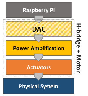
Creating a class to represent a Raspberry Pi digital-to-analog converter is a good example on how to put together the concepts we have been exploring in some of the previous posts. More specifically, DAC with Raspberry Pi and Classes vs. Functions in Python. Besides a Raspberry Pi and a couple of resistors and capacitors, we need an additional DAQ device to calibrate our Pi DAC output.

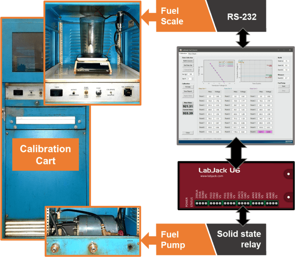
In the post DAC with Raspberry Pi, we used an MCP3008 to measure (and calibrate) the DAC output. This time around I will follow my recommendation of not using the same DAQ to generate and measure the output, using instead a LabJack U3. While a LabJack is not a calibration DAQ device, it is far more accurate than a Pi, therefore moving us in the right direction when it comes to choosing a calibration device.

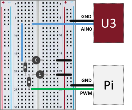
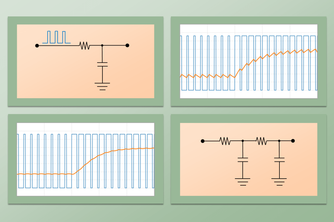
The setup is quite simple: On the Pi side, a GPIO pin used as PWM input to the the low-pass filter and a GND pin. On the U3 side, the RC filter output (which is our DAC output) is connected to the analog input port AIN0, while the GND port is connected to the same GND as the Pi.

The U3 is connected to a separate computer via USB and will be running a variation of the code that can be found on my GitHub page. The Python package that I made containing the LabJack U3 class can be installed from the PyPI (Python Package Index) page.

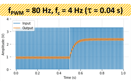
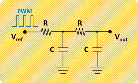
As before, the cascaded second order filter is made of two first order low-pass RC filters, where R = 1 kΩ and C = 10 μF.

Of course, if you don’t have a LabJack, a digital multimeter should do the trick and allow you to measure the DAC output in order to do its calibration. I chose to use a LabJack to gain some insight on the DAC output signal by using its 50 kHz streaming capability (and because an oscilloscope is not among my few possessions).

The next step is to layout what our DAC class should look like. You may want to put down a “skeleton” of the class, as shown below, with a brief description of what the attributes are and what the methods do. Using the reserved word pass allows for placeholders for the methods to be easily created and filled out later.

class DAC:

    def __init__(self):
        # Class constructor
        self._vref = 3.3  # Reference voltage output
        self._slope = 1  # Output transfer function slope
        self._offset = 0  # Output transfer function intercept

    def __del__(self):
        # Class destructor
        # - makes sure GPIO pins are released
        pass

    def reset_calibration(self):
        # Resets the DAC slope and offset values
        pass

    def set_calibratio(self):
        # Sets the DAC slope and offset with calibration data
        pass

    def get_calibration(self):
        # Retrieves current slope and offset values
        pass

    def set_output(self):
        # Sets the DAC output voltage to the desired value
        pass

One of the nice things about using classes is that it’s easy to add (or remove) attributes and methods as you code away. And even better, if you’re using the interactive session of VS Code, saved updates to your methods are immediately reflected in any instance of the class that is present in the session’s “workspace” (to use a MATLAB term, for those familiar with it). In other words, if you were to call that method again using dot notation, it would behave based on the latest modifications that you saved.

In the case of our example, the attributes need to hold the values of a reference voltage (Pi’s 3.3 V if you’re not using any OpAmp with your filter) and the calibration parameters which are used so the DAC can output the correct set voltage value.

from gpiozero import PWMOutputDevice


class DAC:

    def __init__(self, dacpin=12):

        # Checking for valid hardware PWM pins
        if dacpin not in [12, 13, 18, 19]:
            raise Exception('Valid GPIO pin is: 12, 13, 18, or 19')
        # Assigning attributes
        self._vref = 3.3  # Reference voltage output
        self._slope = 1  # Output transfer function slope
        self._offset = 0  # Output transfer function intercept
        # Creating PWM pin object
        self._dac = PWMOutputDevice(dacpin, frequency=700)

    def __del__(self):

        # Releasing GPIO pin
        self._dac.close()

    def reset_calibration(self):
        self._slope = 1
        self._offset = 0

    def set_calibration(self, slope, offset):
        self._slope = slope
        self._offset = offset

    def get_calibration(self):
        print('Slope = {:0.4f} , Offset = {:0.4f}'.format(
            self._slope, self._offset))

    def set_output(self, value):

        # Limiting output
        output = self._slope*value/self._vref + self._offset
        if output > 1:
            output = 1
        if output < 0:
            output = 0
        # Applying output to GPIO pin
        self._dac.value = output

As far as the methods are concerned, a constructor and a destructor, being the latter a good idea so the GPIO pin can be released once you’re done using the class instance. Also, a group of methods to deal with the DAC calibration and a single method to set the DAC output value. Notice that the attribute names start with an underscore. That’s a loose Python convention to define private properties (or methods, if I were to use the underscore as the first character of the method name), unlike other programming languages which are more rigorous about it by making you explicitly define what’s private. The general idea of private properties (or methods) is that they’re not supposed to be accessible directly by the user of the program, therefore, being accessed internally by the code.
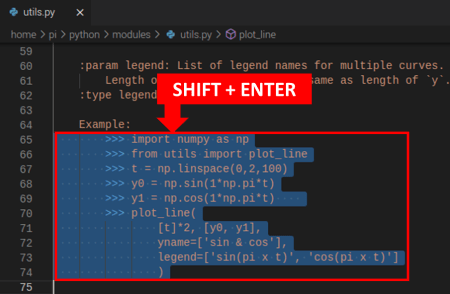
DAC Calibration

First, we create an instance of the DAC class on GPIO pin 18: mydac = DAC(dacpin=18)

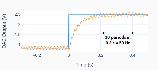
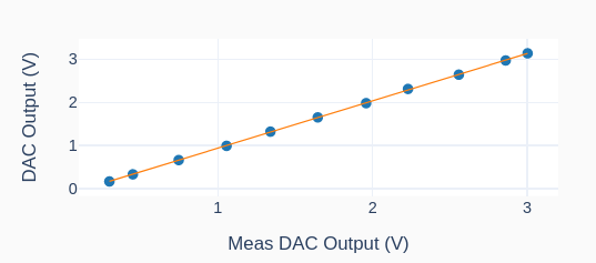
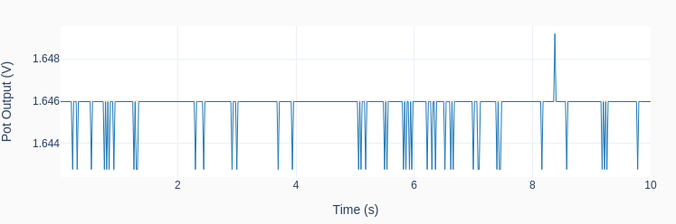
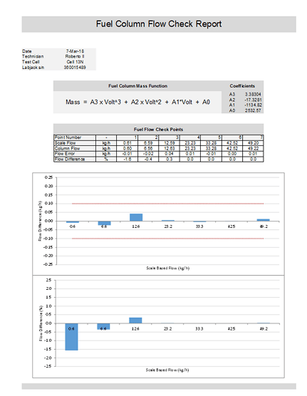
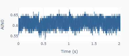
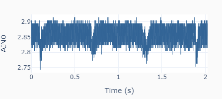
Then, the output calibration is done with two output settings (0.5 and 3.0 V) using the method: mydac.set_output(0.5) and mydac.set_output(3.0). Each time the output is read using the streaming feature of the LabJack U3, as shown on the left. The high frequency noise in the signal is quite apparent and is a most likely due to the limitations of the Raspberry Pi hardware. For the two desired outputs of 0.5 and 3.0 V, the corresponding mean actual values are 0.614 and 2.854 V. Because the system response is linear, two data points are sufficient.

The slope and offset are calculated as slope = (3.0 – 0.5) / (2.854 – 0.614) = 1.116, and offset = 0.5 – (3.0 – 0.5) / (2.854 – 0.614) x 0.614 = -0.185. The calibrated values are applied to the DAC instance using the method mydac.set_calibration(1.116, -0.185). If a new calibration has to be done, the default values of 1 and 0 can be restored by using the method mydac.reset_calibration(). As mentioned earlier, the private attributes _slope and _offset are not dealt with directly by the user but instead through different methods. Of course, in this simple example, they could be changed directly by doing mydac._slope = 1.116 and mydac._offset = -0.185. In more complex situations there might be a few good reasons to avoid direct access to an instance’s attributes.

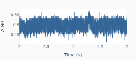
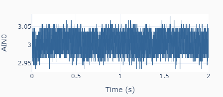
With the calibrated DAC, the new outputs to the same settings as before (0.5 and 3.0 V) give the results on the left, where the actual mean values are 0.493 and 3.006 V, respectively.
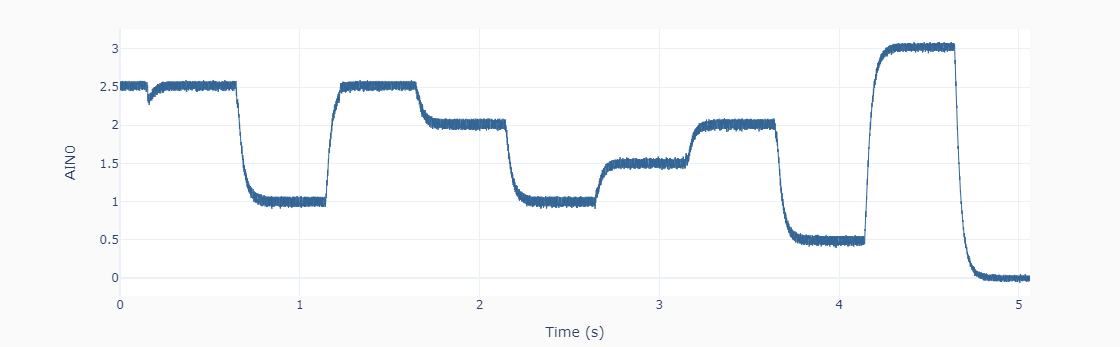
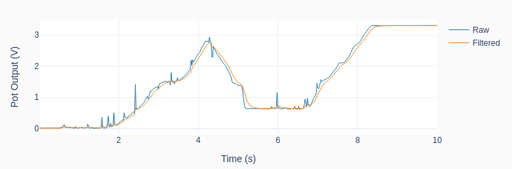
DAC Test

Let’s put the DAC device to the test! The Python code below can be used to generate a random sequence of steps every 0.5 seconds between 0 and 3 V (every 0.5 V). The data is collected using the LabJack U3 streaming feature and plotted in the next figure. Not too bad for our poor man’s DAC.

import time
import numpy as np
from gpiozero_extended import DAC

# Assigning parameter values
tstep = 0.5  # Interval between step changes (s)
tstop = 10  # Total execution time (s)

# Creating DAC object on GPIO pin 18
mydac = DAC(dacpin=18)
mydac.set_calibration(1.116, -0.185)

# Initializing timers and starting main clock
tprev = 0
tcurr = 0
tstart = time.perf_counter()

# Running execution loop
print('Running code for', tstop, 'seconds ...')
while tcurr <= tstop:
    # Updating analog output every `tstep` seconds with
    # random voltages between 0 and 3 V every 0.5 V
    if (np.floor(tcurr/tstep) - np.floor(tprev/tstep)) == 1:
        mydac.set_output(np.round(6*np.random.rand())/2)
    # Updating previous time and getting new current time (s)
    tprev = tcurr
    tcurr = time.perf_counter() - tstart

print('Done.')
# Releasing pin
del mydac
Encoder with Raspberry Pi

Encoder with Raspberry Pi

An encoder or, more specifically, a rotary incremental encoder is a device that can be used to determine incremental changes of the angular position of a rotating shaft. One of the possible hardware constructions is based on a slotted disk attached to the shaft and a pair of optical sensors with a physical offset. The detection of “dark/bright” transitions, as the shaft rotates and the slots pass in front of the sensors, is converted by an electronic circuit into two pulse trains that have a phase shift of 90 degrees between them.

The two signals that are generated by the encoder have to be then processed by a DAQ device, so that the angular increment (or decrement) of the shaft can be determined by “counting the high/low edge transitions” of the two signals. Some DAQ devices have a hardware implementation to deal with encoder signals, thus allowing for much higher shaft speeds. As it is the case of a LabJack.

The Raspberry Pi, on the other hand, doesn’t have the capability to deal with pulse train inputs via hardware. Therefore, it has to rely on a software implementation to do the “edge counting”. We will focus on the class RotaryEncoder in GPIO Zero, which is quite good and very straightforward to use.

To follow along the contents of this post, you may want to review my previous post (H-Bridge and DC Motor with Raspberry Pi), since a motor with an integrated encoder will be used in the examples and, by the end, we will expand the Motor class by adding encoder input capability to it.

From a nomenclature stand point, encoders that produce a pair of square waves (pulse trains) with a 90-degree phase shift are also known as quadrature encoders. However, to take full advantage of this type of encoder, i.e., count all 4 edge transitions during the rotation through one marker (or slot), a hardware-based edge detection is usually required. So, an encoder disc with 45 slots would give a count of 180 effective pulses per revolution (PPR) for a resolution of 2 degrees (360/180). When using a software-based edge detection, the same encoder would have 45 PPR and a resolution of 8 degrees.

The figure below shows typical connections for a Raspberry Pi. Note that the A and B phases are interchangeable. If the pulse count is decreasing when you’re expecting a positive rotation, just swap the connections of the phase wires.

Checking the PPR of the Encoder

After the encoder is connected to the Pi, as shown above, you can use the following Python code to check if the number of Pulses Per Revolution is what you’re expecting. A couple of things will factor into the PPR value.

If the motor has a gear box, the “advertised” PPR value might be incorrect. First of all, understand if the number refers to the quadrature-based value or the marker-based value. Then check if the number is taking into account the gear ratio of the box.

In my case, I am using a motor with a 16 PPR encoder (advertised as a 64 based on a full quadrature implementation) and a gear ratio of 18.8:1. That gives a value of 16 x 18.8 = 300.8 PPR. Ultimately, you can use the sample program below and turn the output shaft by hand to see what you get!

# Importing modules and classes
import time
import numpy as np
from gpiozero import RotaryEncoder

# Assigning parameter values
ppr = 300.8  # Pulses Per Revolution of the encoder
tstop = 20  # Loop execution duration (s)
tsample = 0.02  # Sampling period for code execution (s)
tdisp = 0.5  # Sampling period for values display (s)

# Creating encoder object using GPIO pins 24 and 25
encoder = RotaryEncoder(24, 25, max_steps=0)

# Initializing previous values and starting main clock
anglecurr = 0
tprev = 0
tcurr = 0
tstart = time.perf_counter()

# Execution loop that displays the current
# angular position of the encoder shaft
print('Running code for', tstop, 'seconds ...')
print('(Turn the encoder.)')
while tcurr <= tstop:
    # Pausing for `tsample` to give CPU time to process encoder signal
    time.sleep(tsample)
    # Getting current time (s)
    tcurr = time.perf_counter() - tstart
    # Getting angular position of the encoder
    # roughly every `tsample` seconds (deg.)
    anglecurr = 360 / ppr * encoder.steps
    # Printing angular position every `tdisp` seconds
    if (np.floor(tcurr/tdisp) - np.floor(tprev/tdisp)) == 1:
        print("Angle = {:0.0f} deg".format(anglecurr))
    # Updating previous values
    tprev = tcurr

print('Done.')
# Releasing GPIO pins
encoder.close()

Motor Class with Encoder

The following diagram expands upon the motor setup from the post (H-Bridge and DC Motor with Raspberry Pi). Just as before, we’re using the SN754410 half-bridge chip to set the motor output. But this time around, we can use the encoder to measure the actual shaft angular position and speed.

The Motor class from the post mentioned above can be updated by doing a few modifications to incorporate the rotary encoder.

Besides some new attributes (or properties) used to handle the encoder parameters and its object, two new methods were added: get_angle(), which returns the current encoder angular position in degrees, and reset_angle(), which resets the encoder angle to zero (a handy functionality to have, since we’re using an incremental encoder).

The updated and fully commented class, as well as the rest of the code in this post, can be found on my GitHub page. Also, if you haven’t done it already, I strongly encourage installing VS Code on Raspberry Pi.

Sinusoidal Motor Excitation

The Python program below uses the updated Motor class to run the DC motor with a sinusoidal excitation. Now that we have the encoder capability added to the class, it is possible to measure the angular position of the shaft and calculate its angular velocity. If you’re using VS Code, you must run the code in a terminal instead of an interactive window. The interactive session really competes with the code for CPU resources.

# Importing modules and classes
import time
import numpy as np
from utils import plot_line
from gpiozero_extended import Motor

# Assigning parameter values
T = 2  # Period of sine wave (s)
u0 = 1  # Motor output amplitude
tstop = 2  # Sine wave duration (s)
tsample = 0.01  # Sampling period for code execution (s)

# Creating motor object using GPIO pins 16, 17, and 18
# (using SN754410 quadruple half-H driver chip)
# Integrated encoder is on GPIO pins 25 and 25
mymotor = Motor(
    enable1=16, pwm1=17, pwm2=18,
    encoder1=24, encoder2=25, encoderppr=300.8)
mymotor.reset_angle()

# Pre-allocating output arrays
t = []
theta = []

# Initializing current time step and starting clock
tprev = 0
tcurr = 0
tstart = time.perf_counter()

# Running motor sine wave output
print('Running code for', tstop, 'seconds ...')
while tcurr <= tstop:
    # Pausing for `tsample` to give CPU time to process encoder signal
    time.sleep(tsample)
    # Getting current time (s)
    tcurr = time.perf_counter() - tstart
    # Assigning motor sinusoidal output using the current time step
    mymotor.set_output(u0 * np.sin((2*np.pi/T) * tcurr))
    # Updating output arrays
    t.append(tcurr)
    theta.append(mymotor.get_angle())
    # Updating previous time value
    tprev = tcurr

print('Done.')
# Stopping motor and releasing GPIO pins
mymotor.set_output(0, brake=True)
del mymotor

# Calculating motor angular velocity (rpm)
w = 60/360 * np.gradient(theta, t)

# Plotting results
plot_line([t, t, t[1::]], [theta, w, 1000*np.diff(t)], axes='multi',
          yname=[
              'Angular Position (deg.)',
              'Angular velocity (rpm)',
              'Sampling Period (ms)'])

Once the code finishes running you should get the graph on the bottom left in a web browser page, assuming you ran it in a VS Code terminal. Differently from my other execution loops, I force an execution “pause” by using the command time.sleep(tsample) inside the loop.

By taking that approach, at the expense of a more accurate sampling period, I free up kernel resources to process other interruptions, such as the very CPU-intensive ones coming from the RotaryEncoder. The object is now capable of detecting all the edge transitions coming from the physical encoder, minimizing the number of missed events.

Taking a closer look at the derivative of the angular position (or the velocity) we can detect some fluctuations that are probably due to missed edge counts. The faster the shaft turns, the more likely that is to happen. In our case, 300 PPR at 400 rpm gives 300 x 400 / 60 = 2000 pulses per second. And because the algorithm inside the RotaryEncoder class has to detect all four edge transitions within a pulse, that puts us at 8000 events/sec (or 125 μs/event). Even though the computer is running individual calculations at the nanosecond level, there are many calculations going on inside the algorithm alongside other synchronous tasks. So 125 μs is probably cutting it close.

Still analyzing the results, the sinusoidal PWM excitation will roughly produce a sinusoidal current input to the motor. Since it is the torque, not the angular velocity, that is proportional to the input current, the speed trace will deviate somewhat from the shape of an actual sine wave. That is also quite apparent on the angular position trace, which should be a cosine wave. The deviations with respect to the expected trace shapes are caused mainly by torque being consumed to overcome friction losses in the initial motion and the response time of the motor itself, as a dynamic system.

That is the inherent behavior of this open-loop system. Now that we have the elements in place, by adding the capability to measure the system output, in future posts we’ll explore what can be done by closing the loop on the angular position of the motor shaft.

H-Bridge and DC Motor with Raspberry Pi

H-Bridge and DC Motor with Raspberry Pi

An H-bridge is an electronic circuit that can switch the polarity of the voltage applied to a load. In our case the load is an electric DC motor that is capable of rotating forward and backward. By using a PWM as an input to the system defined by the H-bridge and the motor, we can go from the digital to the analog domain, similarly to what we did with the Raspberry Pi DAC. In this case however, the motor replaces the RC filter and the output is a continuous motor torque/speed instead of a voltage value.

Looking at the bottom half of the diagram introduced in Analog-to-Digital Conversion, the power amplification stage is integrated into the H-bridge and the actuator is the motor. Together they constitute a digital-to-analog converter in a broader sense.

Since the Pi has a limited power output capability, the amplification stage is achieved with an external power supply or a set of batteries that can produce both the higher voltage and current required by a DC motor application. For this post, I’ll use a variable DC power supply set to 12 V and a small DC motor with an integrated encoder. While the encoder won’t be required at this point, it will be used in future posts. And last but not least, there’s the H-bridge, which can be in a single IC chip or part of an IC board. The two types will be considered for some Python code running on a Raspberry Pi 4B.

SN754410 quadruple half-H driver (chip)

The Texas Instruments SN754410 can be used as 4 half-H drivers or 2 H-bridge drivers, depending on the input configuration. The latter can be used to independently control two DC motors with forward and backward rotation. The figure below shows the pins on the chip and the corresponding GPIO pins on the Raspberry Pi.

For a single motor, in addition to the 5V and GND pins, only 3 GPIO pins are required. Unlike the DAC with RC filters, a much lower PWM frequency can be used for the DC motor. Therefore, any 3 GPIO pins can be chosen since the software-implemented PWM at 100 Hz is sufficient.

The breadboard diagram illustrates the wiring for the DC motor control. For example, the Enable signal can be connected to GPIO16, while PWM Forward and PWM Backward could be connected respectively to GPIO17 and GPIO18. The forward speed of the motor is adjusted through the duty cycle of the PWM Forward signal. Correspondingly, the backward speed uses the PWM Backward signal.

Later on in this post, I will go over a Python Class where the three signals can be used to easily set the motor rotation (in an open-loop fashion for now).

L298 dual H-bridge motor speed controller (board)

Another option is to use an IC board which avoids the need of a breadboard and can therefore be used in a more permanent DIY setup. Most importantly, the reason I chose this particular board is that it has a fundamental difference in how the forward and backward rotation is implemented, when compared to the SN754410 chip.

While the wiring is very similar to the previous setup, by taking a closer look (based on the wiring color scheme), you will notice a different number of Enable and PWM signals. This board has 2 Enable signals and only 1 PWM signal. Rotation direction is now controlled with Enable Forward and Enable Backward, while speed is adjusted with a single PWM duty cycle.

Python Motor Class

Even though GPIO Zero has a Motor Class, the class is not ideal for applications where the motor output speed has to continuously transition between forward and backward rotation direction. The Motor Class implemented in the code below allows for that behavior. Additionally, by coding the class from scratch, we can see how the enable and PWM signals are used, as well as how to accommodate for the two types of wiring setup.

If you have been following along on my blog, in one of my previous posts (VS Code on Raspberry Pi) I encourage the creation of a folder dedicated to your Python modules. With that said, this code should be saved in a module named gpiozero_extended.py alongside utils.py in the /home/pi/python/modules folder on your Raspberry Pi. Also, the fully commented Class can be found on my GitHub page.

from gpiozero import DigitalOutputDevice, PWMOutputDevice


class Motor:

    def __init__(self, enable1=None, enable2=None, pwm1=None, pwm2=None):

        # Identifying motor driver type and assigning appropriate GPIO pins
        if pwm1 and pwm2:
            # Driver with 1 enable and 2 PWM inputs
            # Example: SN754410 quadruple half-H driver chip
            if not enable1:
                raise Exception('"enable1" pin is undefined.')
            self._dualpwm = True
            self._enable1 = DigitalOutputDevice(enable1)
            self._pwm1 = PWMOutputDevice(pwm1)
            self._pwm2 = PWMOutputDevice(pwm2)
        elif enable1 and enable2:
            # Driver with 2 enables and 1 PWM input
            # Example: L298 dual H-bridge motor speed controller board
            if not pwm1:
                raise Exception('"pwm1" pin is undefined.')
            self._dualpwm = False
            self._enable1 = DigitalOutputDevice(enable1)
            self._enable2 = DigitalOutputDevice(enable2)
            self._pwm1 = PWMOutputDevice(pwm1)
        else:
            raise Exception('Pin configuration is incorrect.')
        # Initializing output value
        self._value = 0

    def __del__(self):

        # Releasing GPIO pins
        if self._dualpwm:
            self._enable1.close()
            self._pwm1.close()
            self._pwm2.close()
        else:
            self._enable1.close()
            self._enable2.close()
            self._pwm1.close()

    @property
    def value(self):
        return self._value

    @value.setter
    def value(self, _):
        print('"value" is a read only attribute.')

    def set_output(self, output, brake=False):

        # Limiting output
        if output > 1:
            output = 1
        elif output < -1:
            output = -1
        # Forward rotation
        if output > 0:
            if self._dualpwm:
                self._enable1.on()
                self._pwm1.value = output
                self._pwm2.value = 0
            else:
                self._enable1.on()
                self._enable2.off()
                self._pwm1.value = output
        # Backward rotation
        elif output < 0:
            if self._dualpwm:
                self._enable1.on()
                self._pwm1.value = 0
                self._pwm2.value = -output
            else:
                self._enable1.off()
                self._enable2.on()
                self._pwm1.value = -output
        # Stop motor
        elif output == 0:
            if brake:
                if self._dualpwm:
                    self._enable1.off()
                    self._pwm1.value = 0
                    self._pwm2.value = 0
                else:
                    self._enable1.off()
                    self._enable2.off()
                    self._pwm1.value = 0
            else:
                if self._dualpwm:
                    self._enable1.on()
                    self._pwm1.value = 0
                    self._pwm2.value = 0
                else:
                    self._enable1.on()
                    self._enable2.on()
                    self._pwm1.value = 0
        # Updating output value property
        self._value = output

The following example creates a motor object and runs a sinusoidal excitation with an amplitude of 1 for one full period. If you execute the program, you will notice that the direction of the motor rotation changes as the sign of the sine wave changes.

# Importing modules and classes
import time
import numpy as np
from gpiozero_extended import Motor

# Assigning parameter values
T = 4  # Period of sine wave (s)
u0 = 1  # Motor output amplitude
tstop = 4  # Sine wave duration (s)
tsample = 0.01  # Sampling period for code execution (s)

# Creating motor object using GPIO pins 16, 17, and 18
# (using SN754410 quadruple half-H driver chip)
mymotor = Motor(enable1=16, pwm1=17, pwm2=18)

# Initializing current time stamp and starting clock
tprev = 0
tcurr = 0
tstart = time.perf_counter()

# Running motor sine wave output
print('Running code for', tstop, 'seconds ...')
while tcurr <= tstop:
    # Getting current time (s)
    tcurr = time.perf_counter() - tstart
    # Doing I/O every `tsample` seconds
    if (np.floor(tcurr/tsample) - np.floor(tprev/tsample)) == 1:
        # Assigning motor sinusoidal output using the current time stamp
        mymotor.set_output(u0 * np.sin((2*np.pi/T) * tcurr))
    # Updating previous time value
    tprev = tcurr

print('Done.')
# Stopping motor and releasing GPIO pins
mymotor.set_output(0, brake=True)
del mymotor

DC Motor Remarks

If you’re using a motor with an integrated gear box and try some low output values with the motor object, you’ll notice that there’s a dead band where there’s no speed response as the sign changes around small duty cycle values. That happens because it is the DC motor torque (not the angular velocity) that is proportional to the input current (or very simplistically the PWM duty cycle). For small duty cycle values, the torque is being used to overcome the friction losses in the motor bearings and the gear box before the output shaft starts to turn.

There are several low-budget small DC motors that can be purchased online, usually with a wide range of gear ratios for the same overall packaging constraints. There should be an output shaft speed / torque combination that meets your project requirements. Keep in mind that the SN74410 has a limit of 1 Ampère per driver, which might affect the output that can be achieved. Board controllers are generally rated at much higher currents (5 A and above). The power supply capability should also be taken into account, by the way.

Finally, as I mentioned at the top, a motor with an integrated encoder will become essential if we want to incorporate the angular position of the output shaft into the Motor Class. That will enable closed-loop control of the motor speed and/or angular position, making for a good automation example.

Classes vs. Functions in Python

Classes vs. Functions in Python

Using classes (or more broadly object-oriented programming) can really take your coding to the next level. While they can be a bit confusing at first, some of the things you can do with them would be very difficult, if not impossible, to do using function-based programming. A very good and concise definition of classes in Python can be found in the official documentation, which I’ll literally quote below:

“Classes provide a means of bundling data and functionality together. Creating a new class creates a new type of object, allowing new instances of that type to be made. Each class instance can have attributes attached to it for maintaining its state. Class instances can also have methods (defined by its class) for modifying its state.”

If you’re already using functions in Python, moving to classes is a very feasible step. The approach I will take in this post is to compare a class and a set of functions that do the same thing, i.e., some data fitting. As we go over the comparison, I will also be referencing bits and pieces of the quote above, hopefully making it more clear to understand.

First of all, you will want to bundle data and functionality that actually belong together. With that in mind, using classes will actually make sense in the long run.

The attributes is where the data (or states) are kept inside an instance of the class. Because of the nature of classes, each instance exists in the computer memory completely independent of other instances of the same class. In other words, the attributes (or properties) of each instance can hold different values. All instances still contain the same methods of the class. These are actions that can be performed by a given instance that usually modify the attribute values of that particular instance.

If you use functions on a regular basis and look inside a Python class, you’ll recognize that the methods are basically functions. That set of functions that you created to perform related tasks on your data can all be put inside a class. Besides making your code more modular and self-contained, the fact that you can have multiple instances of the same class can come in really handy, as we’ll see later on. All the code in this post can be found on my GitHub page, as well.

Let’s get started on our data fitting code. The data part is a set of ordered (x, y) pairs that will be used in a linear regression. The functionality part is the set of actions that can be performed on the data. More specifically: defining the data points, fitting a line to them, and plotting the original data points and the line of best fit.

As a general grammatical recommendation, variables (or attributes) are substantives, or groups of substantives, since they contain or define something. Variable names such as figuresize, x_values, numdatapoints are all typical in Python.

Since, functions or methods “do something” with “something”, I always start with a verb and then one or more substantives. So, open_figure, define_data, find_data_points are all valid names. It is a convention in Python to use underscores in function or method names. If you use underscores in your variable names, that verb is all you got to quickly distinguish between attributes (variables) and methods (functions) in your code.

Data Fitting Functions

With that said, let’s check below the three (very simple) functions that will be used. One important aspect is that most functions have input arguments and return values. In this simple example, the functions define_data and fit_data return dictionaries containing the output information. In larger projects, functions may be calling functions, who in turn call more functions. Handling and tracking input and output can become pretty complex. By then, most people resort to global variables. Which, in my opinion, should be avoided at all costs. Having local variables that stay local to their functions will make debugging the code much more straightforward.

import numpy as np
import plotly.graph_objects as go
from scipy.stats import linregress


def define_data(x, y, xname=None, yname=None):
    """
    Creates dictionary containing data information.

    """
    if len(x) == len(y):
        data = {
            'xname': xname,
            'yname': yname,
            'x': x,
            'y': y,
        }
    else:
        raise Exception("'x' and 'y' must have the same length.")
    return data


def fit_data(data):
    """
    Calculates linear regression to data points.

    """
    f = linregress(data['x'], data['y'])
    fit = {
        'slope': f.slope,
        'intercept': f.intercept,
        'r2': f.rvalue**2
    }
    print('Slope = {:1.3f}'.format(fit['slope']))
    print('Intercept = {:1.3f}'.format(fit['intercept']))
    print('R-squared = {:1.3f}'.format(fit['r2']))
    return fit


def plot_data(data, fit):
    """
    Creates scatter plot of data and best fit regression line.

    """
    # Making sure x and y values are numpy arrays
    x = np.array(data['x'])
    y = np.array(data['y'])
    # Creating plotly figure
    fig = go.Figure()
    # Adding data points
    fig.add_trace(
        go.Scatter(
            name='data',
            x=x,
            y=y,
            mode='markers',
            marker=dict(size=10, color='#FF0F0E')
        )
    )
    # Adding regression line
    fig.add_trace(
        go.Scatter(
            name='fit',
            x=x,
            y=fit['slope']*x+fit['intercept'],
            mode='lines',
            line=dict(dash='dot', color='#202020')
        )
    )
    # Adding other figure objects
    fig.update_xaxes(title_text=data['xname'])
    fig.update_yaxes(title_text=data['yname'])
    fig.update_layout(
        paper_bgcolor='#F8F8F8',
        plot_bgcolor='#FFFFFF',
        width=600, height=300,
        margin=dict(l=60, r=30, t=30, b=30),
        showlegend=False)
    fig.show()

Below is a little program that uses the three functions to fit some x, y values. Notice how inputs and outputs have to be passed around between functions. Also, if we want to fit a different set of data points, we start carrying around multiple variables in memory, which can eventually be overwritten or confused with something else. By the way, I’m assuming you saved a file named fitfunctons.py in a modules folder which is either on the Python path or is your current working folder.

from modules.fitfunctions import define_data, fit_data, plot_data

# Defining first data set
x1 = [0, 1, 2, 3, 4]
y1 = [2.1, 2.8, 4.2, 4.9, 5.1]
data1 = define_data(x1, y1, xname='x1', yname='y1')
# Fitting data
fit1 = fit_data(data1)
# Plotting results
plot_data(data1, fit1)

# Defining second data set
x2 = [0, 1, 2, 3, 4]
y2 = [3, 5.1, 6.8, 8.9, 11.2]
data2 = define_data(x2, y2, xname='x2', yname='y2')
# Fitting data
fit2 = fit_data(data2)
# Plotting results
plot_data(data2, fit2)

Data Fitting Class

Now let’s take a look at a class (saved in fitclass.py in the same modules folder) that contains the three functions as methods. As far as naming conventions in Python are concerned, classes use UpperCamelCase. Therefore, our class will be called FitData. In addition to the three functions (now as methods inside the class) there’s a constructor method, which is by convention named __init__. It’s in the constructor that we can initialize attributes, in this case the data and fit dictionaries, as well as call other methods. Notice that the first argument to all methods is self, which will hold the pointer to the class instance once that instance is created, and is how attributes and methods are accessed inside the class.

For instance, by passing only self to the fit_data method, I can access any attribute or method of the class by using the self argument with dot notation. For instance, self.data['x'] gets the x values array anytime I need it inside the class.

On the same token, methods don’t need to have return values (although sometimes you may want them to). They can use the self pointer to store the return values as a class attribute. The method fit_data gets the x, y values from the data attribute and stores the fitting parameters in the fit attribute, such as self.fit['slope'] = f.slope.

import numpy as np
import plotly.graph_objects as go
from scipy.stats import linregress


class FitData:
    def __init__(self):
        """
        Class constructor.

        """
        self.data = dict()
        self.fit = dict()

    def define_data(self, x, y, xname=None, yname=None):
        """
        Creates dictionary containing data information.

        """
        if len(x) == len(y):
            self.data['x'] = x
            self.data['y'] = y
            self.data['xname'] = xname
            self.data['yname'] = yname
        else:
            raise Exception("'x' and 'y' must have the same length.")

    def fit_data(self):
        """
        Calculates linear regression to data points.

        """
        f = linregress(self.data['x'], self.data['y'])
        self.fit['slope'] = f.slope
        self.fit['intercept'] = f.intercept
        self.fit['r2'] = f.rvalue**2
        print('Slope = {:1.3f}'.format(self.fit['slope']))
        print('Intercept = {:1.3f}'.format(self.fit['intercept']))
        print('R-squared = {:1.3f}'.format(self.fit['r2']))

    def plot_data(self):
        """
        Creates scatter plot of data and best fit regression line.

        """
        # Making sure x and y values are numpy arrays
        x = np.array(self.data['x'])
        y = np.array(self.data['y'])
        # Creating plotly figure
        fig = go.Figure()
        # Adding data points
        fig.add_trace(
            go.Scatter(
                name='data',
                x=x,
                y=y,
                mode='markers',
                marker=dict(size=10, color='#FF0F0E')
            )
        )
        # Adding regression line
        fig.add_trace(
            go.Scatter(
                name='fit',
                x=x,
                y=self.fit['slope']*x+self.fit['intercept'],
                mode='lines',
                line=dict(dash='dot', color='#202020')
            )
        )
        # Adding other figure objects
        fig.update_xaxes(title_text=self.data['xname'])
        fig.update_yaxes(title_text=self.data['yname'])
        fig.update_layout(
            paper_bgcolor='#F8F8F8',
            plot_bgcolor='#FFFFFF',
            width=600, height=300,
            margin=dict(l=60, r=30, t=30, b=30),
            showlegend=False
        )
        fig.show()

The program below can be contrasted with the one that employed the functions. We can start by creating two instances of the FitData class, which will be two distinct and independent objects in the computer memory. Each instance now holds the self pointer and can therefore access attributes and call methods using dot notation. fitdata1.plot_data() will run that method with whatever attributes are required and that are already stored in that particular instance. Also, print(fitdata2.data) would display the values assigned to the data attribute in the fitdata2 object.

from modules.fitclass import FitData

# Creating class instances
fitdata1 = FitData()
fitdata2 = FitData()

# Defining first data set
x1 = [0, 1, 2, 3, 4]
y1 = [2.1, 2.8, 4.2, 4.9, 5.1]
fitdata1.define_data(x1, y1, xname='x1', yname='y1')
# Fitting data
fitdata1.fit_data()
# Plotting results
fitdata1.plot_data()

# Defining second data set
x2 = [0, 1, 2, 3, 4]
y2 = [3, 5.1, 6.8, 8.9, 11.2]
fitdata2.define_data(x2, y2, xname='x2', yname='y2')
# Fitting data
fitdata2.fit_data()
# Plotting results
fitdata2.plot_data()

You should also observe that all the variables that were being passed around are now incapsulated inside each object, making for code that is more organized and less prone to errors. Of course, these examples are quite simple and keeping track of what’s going on is still pretty straightforward.

Finally, similar to functions, methods can call methods. But since input arguments and return values can all be stored inside the class attributes, nesting method calls becomes much cleaner and easier to do than nesting function calls.

Random Remarks

I was first exposed to Object-Oriented Programming a little over 6 years ago, when I was playing around with a LEGO EV3 Mindstorms. It was in MATLAB, which was my programming language of many, many years. It took me some time to wrap my head around the concept, but once I understood its power, a whole new dimension of programming opened up! I then took to write the code for an entire engine test cell automation system: GUIs, instrumentation interfaces, and everything in between. The level of complexity and modularization that was required in order to succeed was only achievable through the use of classes.

Speaking of GUIs, those are built upon the concept of classes. If you ever venture down that path, there’s another strong reason to learn more and start using them. Once you get it, you’ll never look back.

VS Code on Raspberry Pi

VS Code on Raspberry Pi

When it comes to a Python IDE (Integrated Development Environment) for the Pi, if you want to code like a pro, I would definitely go with Visual Studio Code. It’s free, open source, and runs on pretty much any platform. And no, I’m not getting any kickbacks from Microsoft. While the Raspberry Pi OS installation comes with a couple of IDE options, you will have a more pleasant (and efficient) programming experience if you use VS Code.

Before I go about the installation steps and some useful extensions that can be added, let me first mention two things that I believe can really make a difference for programming in Python: 1) A highly customizable interface that has the same look across different platforms; 2) You can have the editor, the terminal window, AND an interactive Python session all in a single interface. Even more than one instance of each, if that’s the case.

Installing VS Code

First of all, I strongly recommend keeping the default pi username that comes with the Raspberry Pi OS. It has the correct level of administrator privileges and will help keep things communized as we move forward. With that said, open a terminal window on your Pi and run the following commands to make sure the installation is current and to install VS Code:

pi@raspberrypi:~ $ sudo apt update

pi@raspberrypi:~ $ sudo apt install code

That’s pretty much it! But let’s add a few features to make life easier. VS Code allows for a multitude of extensions to be installed. In our case, Python IntelliSense (auto-completion, syntax checking, code formatting) and Jupyter notebook (interactive session, graph renderers) are really useful and should be installed next.

Let’s open VS Code and go to the Extensions Marketplace, as shown in below, and type python in the search bar. Several extensions will show up. Select the Python (Pylance) extension and and install it.

Then type jupyter in the search bar and install the Jupyter Notebook Renderers extension . Sometimes it’s installed automatically when you install the previous extension.

At this point you should be able to see the Python interpreter automatically selected based on the version installed on your Raspberry Pi.

Let’s create our first program in VS Code, which will help understand the layout a bit more and install some additional requirements. As shown next, create a new file from the menu and then select Python as the programming language.

Create a simple program, such as a variation of the famous print('Hello World!'), then right-click anywhere in the editor and select the menu option Run Current File in Interactive Window. That will trigger the installation of the missing piece (ipykernel) required to run interactively.

Accept the prompts that may appear in the lower right corner and/or the main window and wait as the installation opens a new terminal window in VS Code.

Once the installation finishes, the interactive session should be fully enabled and your screen should look somewhat like the one below. You can also type commands in the box at the bottom of the interactive window and execute them by pressing SHIFT + ENTER. For those familiar with MATLAB, the interactive window is very similar to the MATLAB Workspace. You can run bits and pieces of code, try individual commands, and manually inspect variables, among other things.

Installing Plotly

The next step is to install Plotly so we can make some graphs in the interactive window. By the way, I couldn’t find an easy way to have Matplotlib graphs show up in the interactive session in the Raspberry Pi Unix… Besides that, the graphs in Plotly are quite interactive, which is a nice feature to have. So, let’s open a terminal window in VS Code, as shown below:

In the new terminal, do a pip install for Plotly. As you probably realized by now, Python packages can by installed from inside VS Code, without the need to run sudo apt install commands from the standard external Pi terminal.

Finally, for things to work as expected, in the same terminal window, run a pip install for nbformat, a Plotly requirement.

At this point, close and restart VS Code for all the changes to take effect.

Numpy and Personal Preferences

To run some of the examples throughout my blog you will need to install a different version of numpy than the one that comes installed with the Raspberry Pi OS. While it doesn’t replace the original version, the new package will end up installed in the local python site-packages folder, more specifically: /home/pi/.local/lib/python3.9/site-packages. Which version of numpy to choose may be dependent on the Python version that’s running on the Pi. In my case, I run the following command at the VS Code terminal:

python3 -m pip install numpy==1.22

After doing that, numerical library issues will come up, which can be resolved by installing in a Pi terminal:

pi@raspberrypi:~ $ sudo apt-get install libatlas-base-dev

And since you’re at it, you might as well install a useful engineering package (through the VS Code terminal):

python3 -m pip install scipy

I also like to create a folder structure that will explicitly have a modules folder, which will be the location for any Python modules that I create.

That will work well if you use this VS Code settings.json file. It already has the correct folder names and a few more settings for how VS Code should look. You can copy it’s content from my GitHub page and place a file with the exact same name in home/pi/.config/Code/User. The current file in that folder should be empty if you just installed VS Code. In case it isn’t, you may want to save a copy of it with before replacing it with the new one. Open the new file with, yes, VS Code and make sure the Python folder matches the one on your Pi OS installation.

You can also get the keybindings.json file from the GitHub page and place it in the same folder. It allows you to open an interactive session window by pressing ALT+SHIFT+J , as well as to automatically run selected code from the editor in the interactive window by pressing SHIFT + ENTER .

Now it’s a good time to get the plotting function from my post A useful Python plotting module, that I use quite often in the examples, and place it in the correct location with the correct name. Just copy the code from the post and paste it in a new Python file in the VS Code editor. Then save it as utils.py in /home/pi/python/modules/ folder. If you inspect the settings.json file you’ll see that the modules folder is already added to the Python path and it’s content can be imported without any problems.

You can even run the example by selecting the code an hitting SHIFT + ENTER to have it execute in the interactive window. Give it a try!

DAC with Raspberry Pi

DAC with Raspberry Pi

Let’s put some of the concepts from the Digital-to-Analog Conversion post to work with a Raspberry Pi. To get the most out of it, you will need a few resistors and capacitors, as well as an MCP3008. The former will be used to build the low-pass analog filters, while the latter will be used to measure the DAC output. As a general guideline, you don’t want to generate and measure a signal on the same DAQ device, since all sorts of extraneous loops and noise could potentially show up. But because we’re not doing any instrumentation-critical work, we won’t be following that guideline.

The figure shows the layout of the components on a breadboard. The MCP3008 wires will use the same pins that were used in the MCP3008 with Raspberry Pi.

The PWM wire should be connected to GPIO12, which is one of the hardware-implemented PWMs on the Pi (GPIO13, 18, and 19 also have hardware PWM). As a side note, the software-implemented PWM is good for 100 to 200 Hz. The PWM period starts to fall apart above 500 Hz. The hardware PWM can go up to 8 kHz! However, that would be an overkill for our application and we will settle down for a lower value, as shown later on.

It’s also possible to identify on the board two cascaded low-pass RC filters, whose output is connected to pin 1 on the MCP3008 (channel 0 on the GPIO Zero MCP3008 class).

Let’s aim for a step response time (τ) of 0.01 s for our filters. We can then use the formula τ = RC to determine the RC product and choose suitable R and C values. In our case, we should select R = 1 kΩ and C = 10 μF. When putting everything together, make sure the negative side of the capacitors are connected to ground!

The following Python code (mostly derived from the example in Prescribed PWM duty cycle) will run a sequence of PWM duty cycle steps that can be used to better understand the DAC output. Check the list of comments below before digging into the code.

  • Even though the hardware PWM can go up to 8 kHz, it seemed reasonable to use 700 Hz for it. Change this number to lower values (such as 50 Hz) to see the impact on the signal ripple.
  • Both the PWM values as well as the ADC measurements are normalized between 0 and 1 in GPIO Zero. Therefore, they are scaled throughout the code to Vref = 3.3 V.
  • The PWM duty cycle output steps (that correspond to a DAC output) span the entire range. However, the 0 and 1 values are omitted. That’s because they fully bypass the PWM, applying respectively a constant 0 and Vref to the output.
  • Even though the sampling rate of the hardware-based ADC can go up to 6.25 kSamples/s, the signals are sampled at a rate of 500 Samples/s. That’s sufficient for visualization and provides plenty of margin in the execution loop.
import time
import numpy as np
from utils import plot_line
from gpiozero import PWMOutputDevice, MCP3008

# Assigning parameter values
pwmfreq = 700 # PWM frequency (Hz)
pwmvalue = [0.05, 0.2, 0.4, 0.6, 0.8, 0.95, 0.9, 0.7, 0.5, 0.3, 0.1]
tsample = 0.002 # Sampling period for data acquisition (s)
tstep = 0.5 # Interval between PWM output step changes (s)
tstop = tstep * len(pwmvalue) # Total execution time (s)
vref = 3.3  # Reference voltage for the PWM and MCP3008

# Preallocating output arrays for plotting
t = []  # Time (s)
dacvalue = []  # Desired DAC output
adcvalue = []  # Measured DAC output

# Creating DAC PWM and ADC channel (using hardware implementations)
dac0 = PWMOutputDevice(12, frequency=pwmfreq)
adc0 = MCP3008(channel=0, clock_pin=11, mosi_pin=10, miso_pin=9, select_pin=8)

# Initializing timers and starting main clock
tprev = 0
tcurr = 0
tstart = time.perf_counter()

# Initializing other variables used in the loop
count = 1  # PWM step counter
dacvaluecurr = pwmvalue[0]  # Initial DAC output value
dac0.value = dacvaluecurr  # Sending initial value to GPIO pin

# Running execution loop
print('Running code for', tstop, 'seconds ...')
while tcurr <= tstop:
    # Updating PWM output every `tstep` seconds
    # with values from prescribed sequence
    if (np.floor(tcurr/tstep) - np.floor(tprev/tstep)) == 1:
        dacvaluecurr = pwmvalue[count]
        dac0.value = dacvaluecurr
        count += 1
    # Acquiring digital data every `tsample` seconds
    # and appending values to output arrays
    # (values are converted from normalized to 0 to Vref)
    if (np.floor(tcurr/tsample) - np.floor(tprev/tsample)) == 1:
        t.append(tcurr)
        dacvalue.append(vref*dacvaluecurr)
        adcvalue.append(vref*adc0.value)
    # Updating previous time and getting new current time (s)
    tprev = tcurr
    tcurr = time.perf_counter() - tstart

print('Done.')
# Releasing pins
dac0.value = 0
dac0.close()
adc0.close()

# Plotting results
plot_line([t]*2, [dacvalue, adcvalue], yname='DAC Output (V)')
plot_line(t[1::], 1000*np.diff(t), yname='Sampling Period (ms)')

The plots show the output generated using plot_line from the utils.py module. Make sure you have a copy of it that can be imported. Observing the DAC response, it’s possible to notice that for lower PWM duty cycles the stead-state value is higher than the set point. Conversely, a higher duty cycle produces a steady-state value lower than the set point. Later on, we’ll see that it is possible to calibrate the DAC output so a one-to-one relationship can be obtained. It’s also a good practice to plot the actual sampling period that the execution loop is running on. Just to make sure it can keep up.

Output Ripple and Step Response

The next figures show the step response of our Pi DAC for a PWM duty cycle change from 25 to 75 % (0.825 to 2,457 V), respectively for PWM frequencies of 50 and 700 Hz.

For the 50 Hz PWM, the ripple in the output is quite significant and can be easily identified. We can also see that there’s no offset between the desired and the actual steady-state DAC output signals. In the other hand, for the 700 Hz PWM, the ripple in the output is much smaller and isn’t related to the PWM frequency. Unlike the lower frequency case, there’s now an offset between desired and actual outputs.

That offset is mostly caused by the transitions from low-to-high (and vice-versa) in the PWM signal. Because they’re not instantaneous (think of them as very steep ramps instead), the PWM signal going into the low-pass filter will assume values other than low (0V) and high (Vref). These intermediate values become more relevant the higher the frequency is. Interestingly enough, the offset will be zero at 50% duty cycle, regardless of fPWM.

The response time is not affected by the PWM frequency. The theoretical value of 0.02 s (for the combined cascaded low-pass filters used in this example) wasn’t observed on the actual signal. The higher response time of 0.05 s is due in part to the PWM not being a perfectly “square” wave form. One should also speculate other delays in the Raspberry Pi hardware itself, as well as the effect of input/output impedances.

DAC Calibration

The relationship between the set point and the actual analog output values is quite linear and can be determined with the help of a modified version of the Python code above, which also performs a linear regression on the collected data. The code stores (and averages) analog output data for the steady-state portion of every step of the input sequence. The data points are then used in a linear regression to determine the transfer function between desired and actual analog output values. The graphs below show the linear regression and the calibrated output. Check out the code on my GitHub repository for more details.

Final Remarks

While most instrumentation and DAQs these days don’t require analog inputs to do what they’re supposed to do, some of the older pieces of equipment out there still do. Op Amps can be used to expand the output voltage range of our simple Pi DAC to a more common 0 to 5 V.

In this post, I create a DAC class that can be used like any other GPIO Zero class (such as PWMOutputDevice or MCP3008) making it much easier to work with the code. The exercise of building the class also comes in handy as we explore more efficient ways to write DAQ software in Python.

Digital-to-Analog Conversion

Digital-to-Analog Conversion

As the counterpart of analog-to-digital conversion, DAC will take a digital signal and convert it to an analog one. Paraphrasing what I mentioned in previous posts, ADC and DAC walk hand-in-hand bridging the gap between the continuous and discrete domains that modern machines and devices have to deal with.

Even though there are several types of DACs, I will talk about the PWM-based one, where a reference input voltage is switched (in the form of a digital train of pulses) into a low-pass analog filter, producing an analog output. Before we get there, let’s first talk about Pulse Width Modulation, a very clever way to go from the discrete to the continuous domain, invented in the mid-seventies. A PWM signal has two main characteristics: its frequency and its duty cycle.

The figure illustrates the frequency and the concept of duty cycle for a 10 Hz PWM signal. In this case, the period of the PWM is 1/fPWM = 0.1 s. The chosen duty cycle is 25 %, which corresponds to the time the output is “on” (0.025 s). During the remainder of the duration of the PWM period (0.075 s) the output is “off”. As a matter of fact, it’s the modulation of the duty cycle that will control the output level of the DAC system.

Since it’s either fully “on” or fully “off”, the PWM signal is fundamentally a digital one. It’s the frequency and duty cycle of that “on-off” train of pulses, coupled with the response of the sub-system it’s interacting with, that will result in an analog behavior of the output of the overall system, in our case the digital-to-analog converter.

As a side note, the Python code used to generate the graphs in this post can be found on my GitHub page. Make sure to check it out and experiment with the DAC parameters.

The simplest DAC implementation is shown on the left. It consists of a low-pass first-order passive RC filter connected to the PWM output signal Vref. Typically, for a TTL circuit, the voltage can be either 0 (low) or 3.3V (high).

The cutoff frequency (rad/s) of the filter is fc = 1/(RC). Along with the PWM frequency, it can be used to obtain the desired behavior of this simple DAC.

Output Ripple

The PWM signal can be thought as a sequence of low-to-high and high-to-low step inputs into the RC filter. Even with a constantly switching input, this first order system will eventually produce a near constant output. The figures below show the effect of the RC filter cutoff frequency fc as well as the PWM frequency fPWM on the amplitude of the output ripple.

As it can be observed in the plots above, the output voltage will converge to (duty cycle) x Vref , which for the duty cycle of 25 % (used in the example) produces an output of 0.825 V when Vref = 3.3 V. Also, reducing the filter cutoff frequency or increasing the PWM frequency are both effective in reducing the output signal ripple. While having a slow RC filter can greatly reduce the ripple, that will negatively affect the DAC response time when it’s subject to a change in the desired output value.

DAC Step Response

In the case of our DAC, its response time is essentially the response time of the RC filter, i.e. 1/fc = RC (with fc in rad/s). Leaving the details for a future post on analog and digital filtering, for the first order system under consideration, the response time can be defined as the time it takes for the output to reach about 63 % of its final (steady-state) value, after a step input is applied.

The next figure shows how an appropriate combination of a higher PWM frequency and a higher filter cutoff frequency can produce a faster response time, while maintaining roughly the same amplitude of the DAC output ripple. For our example, the response time based on the RC value goes from 0.16 s down to 0.04 s.

Cascaded Filters

The output ripple can be further improved by cascading two first-order RC filters, as shown below. The newly formed second-order filter will have twice the attenuation (dB/decade) above the cutoff frequency. It’s an easy-to-do improvement which is often adopted.

Practical Considerations

Just like its ADC counterpart, DACs also have an inherent quantization in the signal. The digital PWM, generated from the microprocessor clock, has a finite resolution (duty cycle levels) given by the number of bits of the PWM. Typical resolutions range from 8 to 12 bits.

Actual PWM frequencies for DAC devices are much higher than the ones used in the examples above, which were chosen mainly to illustrate the concepts. For applications involving testing of physical systems or automation, frequencies between 500 and 2000 Hz are reasonable. In audio applications, several times the highest frequency of the audible range (20 kHz) seems to be the case. That is, 100 to 200 kHz. However, just as we observed when using higher order filtering, there’s wiggle room to reduce these numbers while still having a good compromise between response time and ripple.

It’s important to make a distinction at this point: if the PWM is used to drive a DC motor directly (or with some power amplification), the motor itself will behave approximately as a first order system. Hence, there’s no need for the RC filter. In this type of application, PWM frequencies of 100 to 200 Hz are just fine.

Amplification of the DAC output beyond the typical 3.3V Vref, can be achieved by using an Op Amp (Operational Amplifier). For a simple non-inverting amplifier, the output voltage is given by:

V2 = V1(1+R1/R2)

By choosing R1 = R2 = 10 kOhm, we can double the output to accommodate a more typical 0 to 5V requirement.

In my next post, we will explore the implementation of a DAC using a Raspberry Pi and a few resistors and capacitors. The Pi has hardware enabled PWM on two of its GPIO pins, which can reach frequencies in the kHz range! That should be an interesting project.

MCP3008 with Raspberry Pi

MCP3008 with Raspberry Pi

Since the Raspberry Pi is fundamentally a digital device, any I/O that is done through it’s GPIO pins will happen through high (one) and low (zero) states. When it comes to input signals that are analog, most likely from a transducer, they need to be converted to the digital domain so the Raspberry Pi can understand them. The MCP3008 is a 10-bit 8-channel analog-to-digital converter chip that has a very straightforward API implementation in GPIO Zero. The MCP3008 device uses an SPI (Serial Peripheral Interface) communication protocol that is fully taken care by the API.

SPI requires four pins for the communication:

  • A “SCLK” pin which provides the clock (pulse train) for the communication.
  • A “MOSI” pin (Master Out, Slave In) which the Pi uses to send information to the device.
  • A “MISO” pin (Master In, Slave Out) which the Pi uses to receive information from the device.
  • A “CEX” pin which is used to start and end the communication with the device, usually for one data sample at a time. Because the Raspberry Pi can have more than one device sharing the same SCLK, MOSI, and MISO pins, the CE0 or CE1 pin will indicate which device to use.

Additionally, the MCP3008 requires two separate voltage inputs ranging from 2.7 to 5.5V. The supply voltage at 5V allows for a higher data sampling rate of 200 kSamples/s (which should be plenty for the Raspberry Pi). A reference voltage of 3.3V improves the absolute resolution to about 3 mV instead of 5 mV since, for a 10-bit device, 1LSB = VREF/1024. However, the choice of VREF also has to satisfy the analog input range requirement of the transducer. If the input is higher that 5V, a resistive voltage divider can be used. Finally, in the case of a Raspberry Pi, both the digital and analog grounds on the device can share the same GND pin.

Important! You must enable the SPI for the MCP3008 communication to work. To do so, go to the Raspberry Pi Configuration menu and select Enable for the SPI in the Interfaces tab.

Hardware vs. Software SPI implementation

The Raspberry Pi has both a hardware and a software implementation of the SPI protocol. It is worth investigating what kind of sampling rates can be achieved with those two types.

The figure on the left shows a comparison between software and hardware implementation results of the sampling period per channel as a function of the number of analog inputs. The code used to collect the data, as well as GPIO pin configurations, can be found on my GitHub page.

For each point on the graph, data was sampled as fast as possible, i.e., with no time step clock, where the only I/O occurring in the execution loop was reading the MCP3008 output. Computational time storing the data in an array was negligible. Not surprisingly, the sampling period increases linearly with the number of input channels and, on my Raspberry Pi 4B, the hardware implementation is in average 3.6 times faster than the software one.

The hardware sampling rate is approximately 6.25 kSamples/s and the software one is approximately 1.72 kSamples/s. Note that it’s common to use Samples (or kSamples) per second for a DAQ device, where the number usually gives the maximum throughput of the device. For example, 5 channels with the hardware implementation still gives 6.25 kSamples/s. However the rate is 1.25 kSamples/s per channel.

Still on the 5 channels example, you can very likely get away without an anti-aliasing filter. Noise above 625 Hz (half of the 1250 Hz sampling rate) should have negligible amplitude and shouldn’t show up as an alias in the actual signal. That doesn’t mean that the analog signal being collected with the MCP3008 doesn’t have (relatively) low frequency noise, which in turn can be filtered using a digital low-pass filter in the DAQ software.

Example with a Potentiometer

A potentiometer is basically a variable resistive voltage divider that will output a voltage between a high and a low voltage value, in our case VREF and GND. Because potentiometers convert a linear or angular position input to a voltage output, they do fall into the transducer category.

In this example, the analog output of the potentiometer will be sampled by the DAQ software. To add a bit of visual excitement, the sampled voltage will be used to change the PWM output that controls the intensity of the LED.

The wires on the right hand side of the figure are all connected to the appropriate pins on the Raspberry Pi. Since hardware SPI will be used:

  • SCLK = GPIO11
  • MISO = GPIO9
  • MOSI = GPIO10
  • CEO = GPIO8

PWM is connected to GPIO16. Note that the LED requires a series resistor, where R can be anywhere between 300 to 1000 Ohm.

Also, pay attention to the semi-circular notch on the MCP3008 chip, so it can be inserted with the right orientation into the breadboard.

The Python code for the example is shown below, where there are a few things worth mentioning:

  • The sampling period is 0.02 s, which gives a sampling rate of 50 Samples/s. That is far below the limit for the hardware SPI implementation (6.25 kSamples/s) and even the software one (1.72 kSamples/s).
  • The execution loop concept with a time step clock is used to ensure a fairly accurate sampling period. Both I/O and computation tasks are performed within a time step with plenty of time to spare.
  • Due to the noise in the analog signal, most likely due to the questionable quality of the potentiometer, a digital low-pass filter is implemented in the code. The cutoff frequency of 2 Hz can be modified for some extra exploration of its effect.
  • For the plotting of the sampled signal to work, a module named utils.py has to be accessible for importing as discussed in my previous post A useful Python plotting module.
import time
import numpy as np
from utils import plot_line
from gpiozero import PWMOutputDevice, MCP3008

# Creating LED PWM object
led = PWMOutputDevice(16)
# Creating ADC channel object
pot = MCP3008(channel=0, clock_pin=11, mosi_pin=10, miso_pin=9, select_pin=8)
# Assining some parameters
tsample = 0.02  # Sampling period for code execution (s)
tstop = 10  # Total execution time (s)
vref = 3.3  # Reference voltage for MCP3008
# Preallocating output arrays for plotting
t = []  # Time (s)
v = []  # Potentiometer voltage output value (V)
vfilt = []  # Fitlered voltage output value (V)
# First order digital low-pass filter parameters
fc = 2  # Filter cutoff frequency (Hz)
wc = 2*np.pi*fc  # Cutoff frequency (rad/s)
tau = 1/wc  # Filter time constant (s)
c0 = tsample/(tsample+tau)  # Digital filter coefficient
c1 = tau/(tsample+tau)  # Digital filter coefficient
# Initializing filter previous value
valueprev = pot.value
time.sleep(tsample)
# Initializing variables and starting main clock
tprev = 0
tcurr = 0
tstart = time.perf_counter()

# Execution loop
print('Running code for', tstop, 'seconds ...')
while tcurr <= tstop:
    # Getting current time (s)
    tcurr = time.perf_counter() - tstart
    # Doing I/O and computations every `tsample` seconds
    if (np.floor(tcurr/tsample) - np.floor(tprev/tsample)) == 1:
        # Getting potentiometer normalized voltage output
        valuecurr = pot.value
        # Filtering value
        valuefilt = c0*valuecurr + c1*valueprev
        # Calculating current raw and filtered voltage
        vcurr = vref*valuecurr
        vcurrfilt = vref*valuefilt
        # Updating LED PWM output
        led.value = valuefilt
        # Updating output arrays
        t.append(tcurr)
        v.append(vcurr)
        vfilt.append(vcurrfilt)
        # Updating previous filtered value
        valueprev = valuefilt
    # Updating previous time value
    tprev = tcurr

print('Done.')
# Releasing pins
pot.close()
led.close()
# Plotting results
plot_line([t]*2, [v, vfilt], yname='Pot Output (V)', legend=['Raw', 'Filtered'])
plot_line([t[1::]], [1000*np.diff(t)], yname='Sampling Period (ms)')

The graphs below show the results of one run on my Raspberry Pi 4B. Observe how the low-pass filter removes the noise from the raw signal as I twirl around the potentiometer knob. That of course comes with a price: the filtered signal now lags the original signal. In DAQ applications where the signal doesn’t need to be filtered in real-time, there are “zero-lag” filtering techniques that can be applied after the signal was acquired. Also note the consistent sampling time step of 20 ms.

A note on Quantization

What would happen if I never touched the potentiometer during the program execution, leaving its output at a constant value? The result is shown in the next graph, where the quantization effect is quite clear on the (very low amplitude) signal noise riding on top of the output voltage. The discrete nature of the output can now be observed, and the values are exactly VREF/210 = 3.3/1024 = 0.0032 V apart!

Analog-to-Digital Conversion

Analog-to-Digital Conversion

Also known as ADC, is the process of converting a physical quantity, usually represented by a voltage at this point, to a set of bits that’s more suitable for a computer to digest. Bearing in mind that the world we live in is analog in nature and the computers we use to interact with it are digital, going from the continuous domain to the discrete domain is an integral part of most machines and devices out there.

Back in the day, when micro-processors and computers weren’t around or were still in their infancy, many systems would function entirely in the analog domain. Take for instance an old record player. From the needle running in the record tracks (a continuous profile of peaks and valleys) to the sound coming out of the speakers, the entire sequence of changes in physical quantities occurred in the analog domain. Nowadays, still on the same example, music is stored as digital content and only converted back to an analog signal when it’s time to make it to the speakers, so we can listen to it with our good old analog ears. This last process of going back from the discrete to the analog domain is handled through a digital-to-analog conversion (DAC) and will be a topic of another post. The entire process can be illustrated with the diagram below.

As I alluded to at the very top, a sensor (or more specifically a transducer) will convert the measured physical quantity to an electrical signal, and ultimately a voltage. The next step in the process is the signal conditioning where some sort of filtering will be applied to the measured voltage. Not only to avoid aliasing, which we will discuss later on, but some times to accomplish other goals, like for example remove a DC component or a very slow drift in the signal.

The next block is the analog-to-digital conversion (ADC), which has mainly two tasks to it: sampling and quantization. Once they are performed, the continuous signal will be broken down into packets of bits that the computer can now handle. We will see that the signal is not only discrete in time but also each sample can only have a finite number of values.

At the bottom half of the diagram is the flip side of the coin: the digital-to-analog (DAC) conversion, an eventual power amplification and, generally speaking, the electro-mechanical actuators.

You should also note that if we are talking about data acquisition only, the focus is the top half of the diagram. If automation is the case, then the entire diagram is in scope.

Sampling

A physical system changes its states continuously over time and it would be impractical to collect continuous data to be used by an inherently discrete system such as the computer. Using the music example, and going back several decades, data would be collected and recorded on magnetic tapes so it could be later edited, mixed, and reproduced. With the computer entering the landscape, those analog systems had their days numbered.

The sampling process occurs in an integrated circuit (IC), where an electronic switch will bring a sample of the signal into the AD converter at a fixed sampling period.

The figure on the right shows 2 seconds of an arbitrary continuous signal sampled at 0.1 seconds (or 10 Hz). The first thing to notice is that we can now store 20 data points instead of an impractical infinite number of continuous points.

There are other considerations that dictate the sampling period (or frequency) than just the amount of data that can be manipulated. The main one is the frequency content of the signal. In other words, how “fast” does the signal change over time. For good signal reconstruction in the time domain, a sampling rate of 10 to 20 times the frequency content of the signal should be used. Most importantly, it must never be below 2 times the highest frequency component of the measured signal. Otherwise, aliasing will potentially occur to the sampled data.

As a quick note, all the plots used in this post were generated using Python and the Matplotlib package. You can get the code on my GitHub page.

Nyquist Theorem and Aliasing

According to the Nyquist sampling theorem, the sampling rate should be at least two times the maximum frequency component of the measured signal. The figure below shows a 20 Hz sinusoidal signal sampled at 21 Hz. Any sampling rate below 40 Hz will result in an alias of the original signal. In this case a new 1 Hz sinusoidal wave will show up.

The frequency of the aliased signals (yes, there’s more than one alias) is not exactly intuitive, as it appears to be in the previous figure. The same original 20 Hz signal sampled at 7 Hz would also produce a 1 Hz aliased signal! Check out the Python code on my GitHub page for a couple of formulas and to explore different sampling rates.

In practical terms, it is hard to guarantee that the signal being sampled won’t contain stray frequencies above the Nyquist frequency. The best way to avoid aliasing is to use an analog low-pass filter before the signal is sampled. Even a simple passive RC filter should suffice, provided a reasonable frequency transition band to accommodate for the poor filter attenuation right above its cut-off frequency.

Back to the music example, audio is usually sampled at 44.1 kHz. Since the human ear can respond to frequencies up to about 20 kHz, sound should be sampled at least at 40 kHz. 44.1 kHz gives a Nyquist frequency of 22.05 kHz and therefore a transition band of 2.05 kHz for a filter with a cut-off frequency of 20 kHz. However, it’s not uncommon to record audio at 48 kHz (or even 96 kHz). The former gives a Nyquist frequency of 24 kHz and therefore a wider 4 kHz transition band for a low-pass filter to attenuate the signal above it’s cut-off frequency of 20 kHz.

For the classically inclined, how does 48 kHz compare with the frequency contents of the music that’s being recorded? A soprano can hit C6 (1046.5 Hz), a violin A7 (3520 Hz), and a piano C8 (4186.01 Hz). Those frequencies are well bellow the Nyquist frequency of 24 kHz and even 10 times (or more) lower than the 48 kHz sampling frequency, allowing also for good signal reconstruction in the time domain.

Quantization

The second task in the AD processing is the quantization of the sampled values. Even though your computer can deal with floating numbers (they’re still a bunch of bits in disguise), the ADC device still ships out a packet of bits for every analog sample. The analog value will be discretized based on a reference voltage and the number of bits used for the quantization.

The ideal transfer function (TF) between the analog input voltage and the digital output code is a straight line where for every possible input there’s a unique output. In other words, the ideal ADC has an infinite resolution. Because the output of the conversion is a digital value, the transfer function of a perfect ADC is in fact a staircase function where each step is 1 LSB (Least Significant Bit).

As shown in the figure, let’s consider the case with a reference voltage VREF = 2 V and a resolution of 3 bits. The step size (1 LSB) is 0.25 V, or in the general case VREF / 2n, where n is the number of bits of the ADC.

Any analog input within a step will be coded to the same digital output. For example, 0.625 to 0.875 V will be coded as 011 (or 3 in decimal representation). Using the reference voltage of 2 V, that would give us 3VREF / 8 = 0.75 V. Therefore, the quantization error goes from +0.125 V to -0.125 V. In other words +/- 0.5 LSB. This would be the case for the perfect ADC shown in the figure, more specifically a single-ended mode configuration with adjusted quantization. A good source explaining other configurations and also sources of errors that occur on an actual ADC can be found here. The full scale (FS in the figure) is VREF – 1LSB, which in the case of this example would be 1.75 V.

If a 4-bit converter is used, the quantization error for the same reference voltage drops to +/- 0.0625 V (still +/- 0.5 LSB) and the FS goes up to 1.875 V.

As we move up in bit resolution, the ADC output starts to approximate the ideal transfer function. In the case of a 10-bit ADC, the quantization error becomes +/- 0.5VREF/1024. Which in our case is approximately +/- 0.001 V, and in the general case +/- 0.05 % of the reference voltage. For a high accuracy 16-bit ADC, the error is approx. +/- 0.0008 % of the reference voltage.

Note that there are additional errors introduced in the quantization process due to offsets, non-linearities, and just noise in general in the electronic circuitry. A 12-bit converter will typically have +/- 0.13 % (instead of +/- 0.012 %) and a 16-bit a typical +/- 0.01%.

Practical Considerations

So, how high should you go with the sampling rate and number of quantization bits? How about the anti-aliasing filter? Keep in mind that faster, higher-resolution hardware comes with a steeper cost. And high sampling rates bring the burden of extra storage space and processing power.

If you are working with audio, definitely 48 kHz and 16-bit ADC for sound recording. 96 kHz (or even 172 kHz) and 24-bit if you’re a pro. And most definitely an anti-alias filter. By the way, the fact that 96 kHz is two times the 48 kHz base rate makes it very easy to down sample a recording for later reproduction: just throw away every other data point.

If you’re toying around with a Raspberry Pi, the sampling rate is the one that suits your needs. For slow changing temperatures 1 Hz is plenty. Pressures maybe 10 to 20 Hz. A 10-bit ADC MCP3008 chip is inexpensive and has plenty of resolution. An anti-aliasing filter is probably overkill. The higher frequency content of noise is also usually low amplitude and therefore shouldn’t affect you signal very much. However, it’s always a good idea to sample your data first at a higher frequency and inspect it as a function of time. Also, be careful with some typical electrical noise like the 60 Hz one caused by the AC outlet.

In a lab or instrumentation setting, 12 to 16-bit and an anti-aliasing filter, such as a simple passive RC one, should be considered. Again, try different sampling rates and filters. As I mentioned before, it’s always important to look at your data as a function of time first with as high as a sampling rate that can be run with the DAQ device at hand. Once you understand what the signal is all about, then a more conscious decision about the hardware requirements can be made.

Finally, just to have some fun with Python, below is the arbitrary signal of this post with two different sampling rates and resolutions. Observe the effects of both the sampling and the quantization on the original signal.

Fuel Flow Measurement (an automation example)

Fuel Flow Measurement (an automation example)

Some of the older engine durability test cells at Navistar needed their fuel consumption measurement system updated. The existing one was built on a dedicated IC board and finding replacement components was becoming increasingly difficult. More importantly, a newer system that was capable of interfacing with other test cell software was also a necessity.

When it comes to automating a measurement system, in addition to the automation of the measurement process itself, two other important tasks have to be kept in mind and automated as well, if possible: the task of checking if the measurement accuracy is within a given specification, and the task of calibrating the system if it is out of spec. These three automation components (the process itself, accuracy checks, and calibration) can be applied to a large group of measurement systems and industrial processes. The fuel flow measurement system belongs to this group.

With that in mind, the fuel flow measurement system consists of two physical parts: a fuel column located in the test cell and a calibration cart. The former performs the measurement task, while the latter the check and calibration tasks. If we remember the post DAQ, SBC, etc., in this particular case, a computer and a DAQ device were used to automate the system. The computer was a very capable test cell PC, that was in charge of controlling many of test cell sub-systems, being the fuel flow measurement system one of them. A single DAQ device (LabJack U6) was part of the test cell hardware and interfaced with the sensors and actuators of both the fuel column and the calibration cart. Below are the main requirements of the automation system:

  • Real-time 10 Hz monitoring of fuel flow (or consumption by the engine)
  • Automatic fuel column refill
  • Capability of manual measurements taken by the operator
  • Capability of measurements commanded by other software via UDP/IP
  • Automated fuel column calibration (fuel mass as a function of voltage)
  • Automated fuel column periodic flow accuracy check
  • Automatic report generation for calibrations and flow checks

Fuel Column

As the engine draws fuel from the column, the output current of the pressure transducer (measured as a voltage over a resistor) is processed by the automation software and a real-time fuel flow value is displayed in the graphical user interface. When the fuel level drops below a certain voltage threshold, the software operates the refill solenoid, topping off the column. This process repeats itself automatically so there’s always fuel in the column.

When a measurement is triggered, either manually or through an external software request, the fuel column is topped off first and then the fuel flow is measured and averaged for a user-defined time duration. The final value is displayed on the interface and sent to the software that made the request, if that’s the case.

An analog input port on the LabJack U6 acquires the voltage signal from the pressure transducer after it’s filtered with an anti-aliasing low-pass filter. The 110 V refill solenoid is switched on or off via a solid-state relay connected to one of the LabJack’s analog output ports.

Calibration Cart

The cart is used to characterize the relationship between the fuel mass in the column and the voltage output from the pressure transducer located at its bottom. When the column is connected to the fuel cart for a calibration procedure, a fuel pump on the cart draws fuel from the column into a container sitting on a high precision scale inside the cart. The automation software executes this procedure automatically by drawing incremental amounts of fuel. At each increment, the fuel mass value is measured by the scale. A function is then fitted to the collected data points of mass vs. voltage.

When the cart is being used to check an existing calibration, the flow measured by the automation software is compared to the fuel flow calculated by using the actual mass collected inside the container on top of the high precision scale, over a certain amount of time.

An analog output port on the LabJack U6 is used to turn the cart pump on or off through a solid-state relay. Communication between the automation software and the fuel scale is done using a RS-232 serial cable connected directly to the test cell PC where the software is installed.

Reporting

Fuel column calibration report example
Fuel column flow check report example

Keeping track of calibrations and flow checks is critical for the engine lab compliance with quality norms and, generally speaking, is an important part of an automated system. To that end, Excel-based reports are automatically generated for each calibration procedure or flow check. These are stored in a database and can be later retrieved and analyzed.

Fuel Column Simulator

Finally, because engine test cells are running most of the time, it was difficult to find a window of opportunity to develop the automation software that controls the fuel column.

To work around this limitation, a fuel column simulator that also includes the calibration cart functionality was created.

Fuel column simulator GUI

The filling and emptying behavior of the column, as well as the other automation system components, was closely matched in the simulator. The main ones were:

  • refill solenoid valve on/off
  • calibration cart pump on/off
  • fuel scale serial communication
  • fuel scale tare operation

Summary

The main idea of this post was to show a real application of the concepts of data acquisition and automation using a computer and a DAQ device. All the elements presented here can be applied to a wide variety of systems. While this one wasn’t too complex, it was part of a larger project to fully automate an engine test cell. Nonetheless, even more complex automation projects can usually be broken down into smaller, more manageable pieces. And that’s how you go about it.

Back to top