Category: Automation

Joystick with Raspberry Pi

Joystick with Raspberry Pi

A two-axis joystick is an input device that can be used to simultaneously control two degrees of freedom of a system, such as roll and pitch on an aircraft, or the X and Y coordinates of a cartesian robot. The Keyestudio KS0008 joystick discussed in this post provides analog signals for the two axis (left-to-right and front-to-back), as well as a digital signal (downward). Like any analog input device used with the Raspberry Pi, the KS0008 requires the MCP3008 analog-to-digital converter chip.

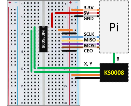
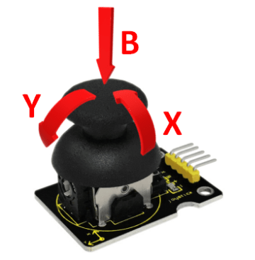
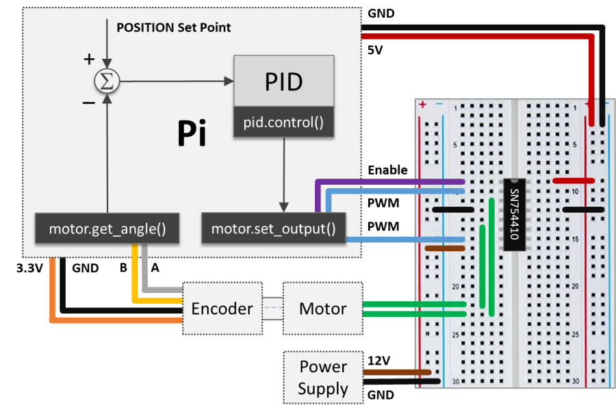
The wiring schematic shows how to connect the joystick to the Pi with the aid of the MCP3008. The analog outputs X and Y are wired to the channels 0 and 1 of the chip. The digital output B can be connected directly to any GPIO pin. In this configuration the KS0008 uses the 3.3V supply voltage. The Python code below samples and displays the three signals in an execution loop.

As a side note, I used the suffix LR (left-to-right) for the joystick’s X axis, and FB (front-to-back) for the Y axis. Mostly to avoid confusion with the digital filter input (X) and output (Y) used later in this post.

# Importing modules and classes
import time
import numpy as np
from gpiozero import MCP3008, DigitalInputDevice

# Creating objects for the joystick outputs
joyLR = MCP3008(channel=0, clock_pin=11, mosi_pin=10, miso_pin=9, select_pin=8)
joyFB = MCP3008(channel=1, clock_pin=11, mosi_pin=10, miso_pin=9, select_pin=8)
joyB = DigitalInputDevice(18)
# Assigning some parameters
tsample = 0.02  # Sampling period for code execution (s)
tdisp = 0.5  # Output display period (s)
tstop = 30  # Total execution time (s)
vref = 3.3  # Reference voltage for MCP3008

# Initializing variables and starting main clock
tprev = 0
tcurr = 0
tstart = time.perf_counter()
# Running execution loop
print('Running code for', tstop, 'seconds ...')
while tcurr <= tstop:
    # Getting current time (s)
    tcurr = time.perf_counter() - tstart
    # Doing I/O and computations every `tsample` seconds
    if (np.floor(tcurr/tsample) - np.floor(tprev/tsample)) == 1:
        # Getting joy stick normalized voltage output
        valLRcurr = joyLR.value
        valFBcurr = joyFB.value
        # Calculating current time raw voltages
        vLRcurr = vref*valLRcurr
        vFBcurr = vref*valFBcurr
        # Getting the Z axis state
        Bcurr = joyB.value
        # Displaying output voltages every `tdisp` seconds
        if (np.floor(tcurr/tdisp) - np.floor(tprev/tdisp)) == 1:
            print("X = {:0.2f} V , Y = {:0.2f} V , B = {:d}".
            format(vLRcurr, vFBcurr, Bcurr))
    # Updating previous time value
    tprev = tcurr

print('Done.')
# Releasing pins
joyLR.close()
joyFB.close()
joyB.close()

The interactive window output in VS Code should look something like what’s shown next. Note that the center position of the joystick outputs approximately half of the 3.3V supply voltage, i.e., 1.65V. Also observe the change in the B digital value as the joystick is pressed.

Running code for 30 seconds ...
X = 1.64 V , Y = 1.64 V , B = 0
X = 3.30 V , Y = 3.30 V , B = 0
X = 3.30 V , Y = 3.08 V , B = 0
X = 1.65 V , Y = 1.65 V , B = 0
X = 1.64 V , Y = 1.65 V , B = 1
X = 1.64 V , Y = 1.64 V , B = 1
X = 1.64 V , Y = 1.64 V , B = 0
X = 1.00 V , Y = 1.64 V , B = 0
X = 0.01 V , Y = 1.64 V , B = 0
X = 0.00 V , Y = 1.64 V , B = 0
X = 1.64 V , Y = 1.64 V , B = 0
X = 1.63 V , Y = 1.35 V , B = 0
X = 1.64 V , Y = 0.00 V , B = 1
X = 1.63 V , Y = 0.00 V , B = 1
X = 1.64 V , Y = 0.00 V , B = 0
X = 1.64 V , Y = 1.64 V , B = 0
...
X = 1.48 V , Y = 0.34 V , B = 0
X = 1.22 V , Y = 0.00 V , B = 0
X = 1.23 V , Y = 0.00 V , B = 0
Done.

Joystick Output Filtering

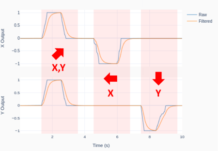
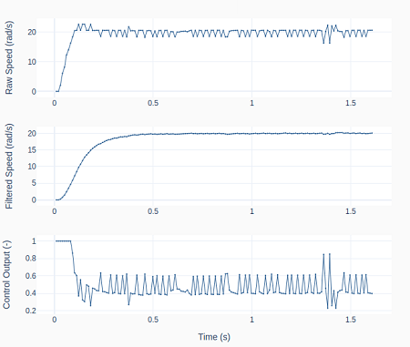
Eventually, the joystick output signal can be a bit jittery, due to the fact that not all of us are born with perfect control over our thumb motion.

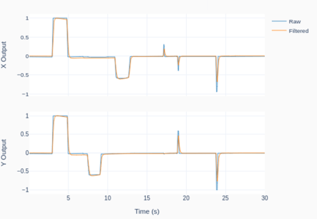
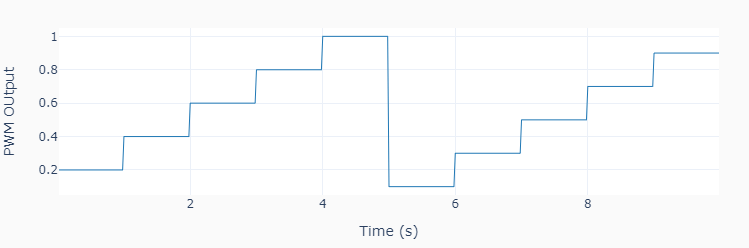
The plot was generated using the Python code below, where a digital low-pass filter with a cutoff frequency of 1Hz was applied to the joystick X and Y output signals. Of course, the cutoff frequency has to be adjusted based on the desired overall system response, which includes what the joystick is controlling.

The outputs were also normalized between -1 and 1. While any transfer function can be designed to map the original 0 to 3.3V range, -1 to 1 seems appropriate if a DC motor is being controlled between full speed reverse and full speed forward.

# Importing modules and classes
import time
import numpy as np
from utils import plot_line
from gpiozero import MCP3008

# Creating ADC channel objects for the joystick inputs
joyLR = MCP3008(channel=0, clock_pin=11, mosi_pin=10, miso_pin=9, select_pin=8)
joyFB = MCP3008(channel=1, clock_pin=11, mosi_pin=10, miso_pin=9, select_pin=8)
# Assigning some parameters
tsample = 0.02  # Sampling period for code execution (s)
tstop = 10  # Total execution time (s)
vref = 3.3  # Reference voltage for MCP3008
# Preallocating output arrays for plotting
t = []  # Time (s)
xLRn = []  # Joy stick X direction output (-1 to 1)
xFBn = []  # Joy stick Y direction output (-1 to 1)
yLRn = []  # Filtered X direction output (-1 to 1)
yFBn = []  # Filtered Y direction output (-1 to 1)

# First order digital low-pass filter parameters
fc = 1  # Filter cutoff frequency (Hz)
tau = 1/(2*np.pi*fc)  # Filter time constant (s)
# Filter difference equation coefficients
a1 = -tau/(tsample+tau)
b0 = tsample/(tsample+tau)
# Initializing filter values
xLR = [joyLR.value]  # x[n]
xFB = [joyFB.value]  # x[n]
yLR = xLR * 2  # y[n], y[n-1]
yFB = yLR * 2  # y[n], y[n-1]
time.sleep(tsample)

# Initializing variables and starting main clock
tprev = 0
tcurr = 0
tstart = time.perf_counter()
# Running execution loop
print('Running code for', tstop, 'seconds ...')
while tcurr <= tstop:
    # Getting current time (s)
    tcurr = time.perf_counter() - tstart
    # Doing I/O and computations every `tsample` seconds
    if (np.floor(tcurr/tsample) - np.floor(tprev/tsample)) == 1:
        # Getting joy stick normalized voltage output
        xLR[0] = joyLR.value
        xFB[0] = joyFB.value
        # Filtering signals
        yLR[0] = -a1*yLR[1] + b0*xLR[0]
        yFB[0] = -a1*yFB[1] + b0*xFB[0]
        # Updating output arrays with normalized output
        t.append(tcurr)
        xLRn.append(-1 + 2*xLR[0])
        xFBn.append(-1 + 2*xFB[0])
        yLRn.append(-1 + 2*yLR[0])
        yFBn.append(-1 + 2*yFB[0])
        # Updating previous filter output values
        yLR[1] = yLR[0]
        yFB[1] = yFB[0]
    # Updating previous time value
    tprev = tcurr

print('Done.')
# Releasing pins
joyLR.close()
joyFB.close()
# Plotting results
plot_line([t]*2, [xLRn, yLRn], yname='X Output', legend=['Raw', 'Filtered'])
plot_line([t]*2, [xFBn, yFBn], yname='Y Output', legend=['Raw', 'Filtered'])

A Note on Joystick Drift

Even though the KS0008 that I used didn’t have a noticeable drift, it is possible that the output values at the “center position” can drift over time. This means that, over time, your system may start moving around, even when it’s supposed to be at rest at the joystick’s “center position”.

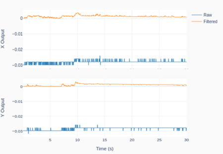
One way to address the issue is to use a digital band-pass filter, which attenuates both the low and high frequency content of a signal. Since the lower cutoff frequency will remove the DC component of the signal (the value that is held constant), it has to be chosen carefully depending on the application. If you are controlling an RC car (where there are extended periods of wide-open-throttle conditions), the band-pass filter may start attenuating the WOT value, causing the car to slow down! On the other hand, if you are controlling a drone, where zero-position drifts are highly undesirable, the band-pass filter may be what you need, since there are no extended periods of moving forward-backward or side-to-side.

The following Python program implements a digital first-order band-pass filter for the joystick outputs, with low and high cutoff frequencies respectively of 0.005 and 2 Hz. The plots show the joystick’s X-Y motion traces for 30 seconds, as well as the “center-position” rest case. The latter helps illustrate how the DC component of the signal is almost fully removed.

# Importing modules and classes
import time
import numpy as np
from utils import plot_line
from gpiozero import MCP3008

# Creating ADC channel objects for the joystick inputs
joyLR = MCP3008(channel=0, clock_pin=11, mosi_pin=10, miso_pin=9, select_pin=8)
joyFB = MCP3008(channel=1, clock_pin=11, mosi_pin=10, miso_pin=9, select_pin=8)
# Assigning some parameters
tsample = 0.02  # Sampling period for code execution (s)
tstop = 30  # Total execution time (s)
vref = 3.3  # Reference voltage for MCP3008
# Preallocating output arrays for plotting
t = []  # Time (s)
xLRn = []  # Joy stick X direction output (-1 to 1)
xFBn = []  # Joy stick Y direction output (-1 to 1)
yLRn = []  # Filtered X direction output (-1 to 1)
yFBn = []  # Filtered Y direction output (-1 to 1)

# First order digital band-pass filter parameters
fc = np.array([0.005, 2])  # Filter cutoff frequencies (Hz)
tau = 1/(2*np.pi*fc)  # Filter time constants (s)
# Filter difference equation coefficients
a0 = tau[0]*tau[1]+(tau[0]+tau[1])*tsample+tsample**2
a1 = -(2*tau[0]*tau[1]+(tau[0]+tau[1])*tsample)
a2 = tau[0]*tau[1]
b0 = tau[0]*tsample
b1 = -tau[0]*tsample
# Assigning normalized coefficients
a = np.array([1, a1/a0, a2/a0])
b = np.array([b0/a0, b1/a0])
# Initializing filter values
xLR = [joyLR.value] * len(b)  # x[n], x[n-1]
xFB = [joyFB.value] * len(b)  # x[n], x[n-1]
yLR = [0] * len(a)  # y[n], y[n-1], y[n-2]
yFB = [0] * len(a)  # y[n], y[n-1], y[n-2]
time.sleep(tsample)

# Initializing variables and starting main clock
tprev = 0
tcurr = 0
tstart = time.perf_counter()
# Running execution loop
print('Running code for', tstop, 'seconds ...')
while tcurr <= tstop:
    # Getting current time (s)
    tcurr = time.perf_counter() - tstart
    # Doing I/O and computations every `tsample` seconds
    if (np.floor(tcurr/tsample) - np.floor(tprev/tsample)) == 1:
        # Getting joy stick normalized voltage output
        xLR[0] = joyLR.value
        xFB[0] = joyFB.value
        # Filtering signals
        yLR[0] = -np.sum(a[1::]*yLR[1::]) + np.sum(b*xLR)
        yFB[0] = -np.sum(a[1::]*yFB[1::]) + np.sum(b*xFB)
        # Updating output arrays with normalized output
        # (The filtered values have no DC component)
        t.append(tcurr)
        xLRn.append(-1 + 2*xLR[0])
        xFBn.append(-1 + 2*xFB[0])
        yLRn.append(2*yLR[0])
        yFBn.append(2*yFB[0])
        # Updating previous filter output values
        for i in range(len(a)-1, 0, -1):
            yLR[i] = yLR[i-1]
            yFB[i] = yFB[i-1]
        # Updating previous filter input values
        for i in range(len(b)-1, 0, -1):
            xLR[i] = xLR[i-1]
            xFB[i] = xFB[i-1]
    # Updating previous time value
    tprev = tcurr

print('Done.')
# Releasing pins
joyLR.close()
joyFB.close()
# Plotting results
plot_line([t]*2, [xLRn, yLRn], yname='X Output', legend=['Raw', 'Filtered'])
plot_line([t]*2, [xFBn, yFBn], yname='Y Output', legend=['Raw', 'Filtered'])
Motor Position Control with Raspberry Pi

Motor Position Control with Raspberry Pi

Along the lines of the Motor Speed Control post, let’s reuse some of our Python classes to control the angular position of a DC motor. We’ll also look into how to tune the PID using the Ziegler-Nichols method, as well as different ways to apply a position set point input.

Like before, the starting point is the Raspberry Pi setup that can handle both a PWM output and an encoder input. Unlike the speed control scenario, there’s no need to calculate and filter the speed from the measured angular position.

Most of the work presented in this post was done using the Python code below. It uses the Motor class and the Digital PID class as its building blocks. On my GitHub page, you can find the complete version of this program, a slight variation of it (used for the PID tuning), and all the classes that it uses.

# Importing modules and classes
import time
import numpy as np
from gpiozero_extended import Motor, PID

# Setting general parameters
tstop = 1  # Execution duration (s)
tsample = 0.01  # Sampling period (s)
thetamax = 180  # Motor position amplitude (deg)

# Setting motion parameters
# (Valid options: 'sin', 'cos')
option = 'cos'
if option == 'sin':
    T = 2*tstop  # Period of sine wave (s)
    theta0 = thetamax  # Reference angle
elif option == 'cos':
    T = tstop  # Period of cosine wave (s)
    theta0 = 0.5*thetamax  # Reference angle

# Creating PID controller object
kp = 0.036
ki = 0.379
kd = 0.0009
taupid = 0.01
pid = PID(tsample, kp, ki, kd, tau=taupid)

# Creating motor object using GPIO pins 16, 17, and 18
# (using SN754410 quadruple half-H driver chip)
# Integrated encoder on GPIO pins 24 and 25.
mymotor = Motor(
    enable1=16, pwm1=17, pwm2=18,
    encoder1=24, encoder2=25, encoderppr=300.8)
mymotor.reset_angle()

# Initializing variables and starting clock
thetaprev = 0
tprev = 0
tcurr = 0
tstart = time.perf_counter()

# Running execution loop
print('Running code for', tstop, 'seconds ...')
while tcurr <= tstop:
    # Pausing for `tsample` to give CPU time to process encoder signal
    time.sleep(tsample)
    # Getting current time (s)
    tcurr = time.perf_counter() - tstart
    # Getting motor shaft angular position
    thetacurr = mymotor.get_angle()
    # Calculating current set point angle
    if option == 'sin':
        thetaspcurr = theta0 * np.sin((2*np.pi/T) * tcurr)
    elif option == 'cos':
        thetaspcurr = theta0 * (1-np.cos((2*np.pi/T) * tcurr))
    # Calculating closed-loop output
    ucurr = pid.control(thetaspcurr, thetacurr)
    # Assigning motor output
    mymotor.set_output(ucurr)
    # Updating previous values
    thetaprev = thetacurr
    tprev = tcurr

print('Done.')
# Stopping motor and releasing GPIO pins
mymotor.set_output(0, brake=True)
del mymotor

PID Tuning using Ziegler-Nichols

Unfortunately, the PID tuning method presented in the previous post cannot be used to obtain an initial set of controller gains. The first-order approximation used for the speed response doesn’t work for the angular position, since it increases linearly once a steady-state speed is reached. In other words, the DC motor system with position as an output is an integrator of the corresponding system with speed as an output.

That brings us to the Ziegler-Nichols method, which can be used with a closed-loop system. In our case, the feedback loop is closed on the motor shaft position. The method is based on starting the tuning process only with a proportional gain and then increasing its value, until the closed-loop system becomes marginally stable. I.e., oscillates with a constant amplitude. The four plots below show the response and corresponding controller output for increasing values of.

The first question that comes to mind is what should the starting value ofbe. A good guess is based on the size of the step input and the saturation limit of the controller. The very instant the step input is applied, the position error going into the controller is equal to the step size. Therefore, at that moment, the controller output is given by . As shown in the first plot, for , the initial controller output is 0.6 for a step input of 20 degrees. The choice of the step size and the initial proportional gain are such that the controller doesn’t saturate (in our case, 1 is the output limit) and there’s still room to increase the gain without running “too much” into the saturation zone.

The ultimate proportional gainis achieved when the system oscillates with a constant amplitude. In our example, . Under this condition, the ultimate oscillation period can be extracted from the last plot above and is calculated as.

The Ziegler-Nichols method states that for a 1/4 decay ratio of the closed-loop system response, the PID gains are given by:

The graph shows the closed-loop response for a shaft position step input of 60 degrees. The PID gains were obtained after substitutingandinto the formulas above.

Observe the 1/4 decay ratio of the amplitude. Also, the fact that the motor position cannot meet exactly 60 degrees causes the integral error to build up, resulting in small position “jumps” around the 1.4 and 1.7 s marks.

Starting from the gains defined by using the Ziegler-Nichols method, let’s do some manual tuning aiming to decrease the oscillation of the closed-loop response. That can be achieved by decreasing the integral gain and increasing the derivative gain.

The plot on the left shows the system response for values that were obtained after a few attempts. The idea is to later compare the effect of the two sets of gains on the response (when applying different types of position set point inputs).

Sine and Cosine Path Functions

While using step changes to move from one position to another is fine, there are situations where we want the position to follow a pre-determined path. By choosing the right combination of PID gains and characteristics of the path function, it’s possible to greatly improve the tracking ability of the position controller.

In this post let’s take a look at two trigonometric functions (sine and cosine), that can be used to move the motor to a given set point angle and then back to its initial position. By inspecting the code above, we can identify the sine and cosine path functions shown below.

and

By choosing suitable values of the amplitudeand period, the two functions can produce motion paths that have the same set point (maximum) angle and the same motion duration to return to the original angular position.

The next two plots show the general closed-loop tracking performance for the sine-based path function, using the two sets of PID gains obtained in the previous section. Notice the more pronounced oscillatory behavior for the more aggressive set of gains. Additionally, due to the nature of the sine-based path, the initial and final speeds are not zero.

The cosine-based path function on the other hand (shown below) has zero initial and final speeds. That characteristic can greatly reduce the system oscillation, especially at the very beginning of the motion.

Final Remarks

When it comes to position control, the DC motor is usually part of a machine or even a robot, where it is important to understand the dynamic behavior of the complete system. Speed and accuracy are usually conflicting goals that have to be compromised to obtain the best performance of the closed-loop control system. However, having a suitable path function can minimize undesired system oscillation caused by the input excitation (or path).

In future posts we will take a deeper look into path functions, particularly the ones that in addition to having zero end-point speeds also have zero end-point accelerations. Stay tuned!

PID Tuning

PID Tuning

Tuning a PID controller consists of choosing the best values for the proportional, integral, and derivative gains in order to satisfy some performance criteria of the closed-loop system. If we’re able to characterize or model the plant that we want to control, then it’s possible do find the best gains either through direct calculation or through simulation.

If we go back to the day when computers weren’t exactly around and there was no such thing as a digital PID, folks had to come up with methods that could be applied directly to the plant or process. Developed respectively in the 1940s and 50s, the well known Ziegler-Nichols and Cohen-Coon methods were the way to go about PID tuning back then. One problem with those two methods is that they result in a fairly aggressive set of gains that can potentially lead to an unstable (or a reduced stability margin) closed-loop system. That undesired characteristic becomes even more critical when a digital PID is employed.

Because we will be dealing mostly with DC motors, I’ll go over a method where the motor speed response is approximated by a first order system. The identified open-loop system is then used to determine the PID gains for the corresponding closed-loop system. In a future post we will go over characterizing the motor individual plant parameters, thus obtaining a better model.

So, let’s try to keep the math under control and start with characterization of the first-order system.

First-Order System

If we look back at the digital filter post, we can extend the low-pass filter equation to a more general form of the first-order system, given by:

where the steady-state gainis the ratio between system output and input. As seen in that same post,is the response time of the system. By determining those two parameters, the first-order system can be fully characterized.

Closed-Loop System

The block diagram below represents the closed-loop system with a PID controller and our first-order system, the latter now expressed as a differential equation. While technically correct, no one uses a time-based representation of the system as shown in the diagram. Mostly because it is really difficult to work with differential equations whose inputs and outputs are all interconnected in some way.

Thankfully, a pretty smart guy named Pierre-Simon Laplace (1749 – 1827) came up with the Laplace transform. It allows for mere mortals to treat complicated convolution problems involving differential equations as simple algebraic ones. We can then redraw the diagram using the corresponding Laplace transforms, as shown in the more familiar form below.

Because we will be doing some algebraic manipulation let’s use the following transfer function notation:

Where

and

Doing the usual “with a few steps, it can be shown that” the closed-loop system transfer function in our case is:

It has the characteristic equation of a second-order system, with damping ratio(zeta) and natural frequency

or

Where

and

After all this mumbo jumbo, we’re finally getting to a point where, for a given first-order plant (with knownand), we can determine the PID gains,andthat would give us the desired closed-loop response, characterized byand. In other words, by selecting a damping ratio and a natural frequency, we can determine a set of PID gains that make our closed-loop system behave as desired.

PID Gains Selection

If we take a look at the last two equations, there are three unknowns (the PID gains) for two known parameters (and ). A good starting point is to make . That way, we can solve the two following equations, for and.

and

Where:

  • in rad/s is the natural frequency of the closed-loop system. The larger its value the faster the system’s response time. In practical terms, you cannot make this number arbitrarily high since you may run into saturation of the controller output. While, for most applications, short saturation periods are fine, it’s better to keep them at a minimum.
  • is the damping ratio of the closed-loop system. Values close to 1 (critical damping ratio) will keep the oscillations and overshoot to a step input under control. In some closed-loop positioning applications, overshoot isn’t an option. Hence, a damping ratio greater than 1 is required.

Finally, note that the PID gains should always be positive. Therefore,.

DC Motor PID Tuning

It’s time to use the hardware setup and code from the Motor Speed Control post to do some exploration of this PID tuning method. First, a step input is applied to the open-loop motor in order to determine the first order response parametersand.

For our little DC motor, with the Raspberry Pi setup, the steady state gain is 20.9/0.5 = 41.8 rad/s/u. Remember that, in our case, u is the normalized PWM output between -1 and 1. The response time of the open-loop system is 0.184 s.

To improve the parameter extraction, a zero-phase filter was used. The code that automatically determines the parameters from the system response can be found on my GitHub page.

Next step consists of choosing values for the closed-loop system’s natural frequencyand damping ratio. The graphs on the left show the system response to a step input for a natural frequency of 2 Hz () and. Using the last two formulas for the integral and proportional gains

,

with all the values we gathered so far, would result inand. We can observe that the motor now takes 0.11 s to reach the target speed (instead of 0.184 to reach 63% of it). That comes of course at expense of using the full capacity of the PWM with some brief saturation.

The reasoning behind my choice ofandis that I wanted a faster response with limited saturation. 2 Hz was the right amount for that. I also wanted a damping ratio slightly greater than one to avoid any oscillations. At this point you might be asking yourself: why is the closed-loop response showing an oscillatory behavior then! The answer is a combination of:

  • The motor is in fact a second order system, not a first order one as our approximation suggests. So, higher order modes may start showing up in the closed-loop response
  • The PID is discrete, not continuous (as that was the basis for all the deductions above). And we’ve seen that the digitalization of the PID tends to promote a more oscillatory behavior
  • The actual closed-loop system includes the transfer function of a low-pass filter for the motor speed. So, the overall system is not composed only by a PID and a plant, as we initially assumed.

Acknowledging that the choice of gains was fairly straightforward, the resulting closed-loop response is quite good! And we haven’t incorporated the derivative gain yet. While it’s usage is not always necessary, it tends to be quite helpful in the case of closed-loop DC motor control. A good starting point foris a couple of orders of magnitude smaller than the proportional gain. So, after starting with 0.001, I ended up with a value of 0.005. The addition of the derivative term really decreased the overshoot and virtually removed the oscillations.

Finally, the next set of graphs shows the results when choosing different natural frequencies and damping ratios. Notice the effect on the response time, the overshoot and the saturation of the controller output.

Motor Speed Control with Raspberry Pi

Motor Speed Control with Raspberry Pi

Let’s use the Motor class with encoder and the Digital PID class to create a closed-loop speed controller for a DC motor. Those two classes have all the required attributes and methods that we need to program an execution loop for a PID controller with very few lines of code.

The starting point is the Raspberry Pi setup that was used to implement encoder capability into the Motor class. I took the artistic liberty to create the diagram below, where I combine visual elements of the PID loop, the hardware connections, and the class methods used for the I/O between the Pi computer and the physical system.

Going back to the concept of execution loops, the I/O tasks are taken care by the Motor class methods get_angle() and set_output(). The computation tasks happening in between are essentially the shaft speed calculation, low-pass filtering, and PID control action. The Python code below implements the execution loop, where the different elements in the Pi box above can be identified. The complete program, which includes the plotting features, along with the Python module with all necessary classes, can be found on my GitHub page.

# Importing modules and classes
import time
import numpy as np
from gpiozero_extended import Motor, PID

# Setting general parameters
tstop = 2  # Execution duration (s)
tsample = 0.01  # Sampling period (s)
wsp = 20  # Motor speed set point (rad/s)
tau = 0.1  # Speed low-pass filter response time (s)

# Creating PID controller object
kp = 0.15
ki = 0.35
kd = 0.01
taupid=0.01
pid = PID(tsample, kp, ki, kd, umin=0, tau=taupid)

# Creating motor object using GPIO pins 16, 17, and 18
# (using SN754410 quadruple half-H driver chip)
# Integrated encoder on GPIO pins 24 and 25.
mymotor = Motor(
    enable1=16, pwm1=17, pwm2=18,
    encoder1=24, encoder2=25, encoderppr=300.8)
mymotor.reset_angle()

# Initializing previous and current values
ucurr = 0  # x[n] (step input)
wfprev = 0  # y[n-1]
wfcurr = 0  # y[n]

# Initializing variables and starting clock
thetaprev = 0
tprev = 0
tcurr = 0
tstart = time.perf_counter()

# Running execution loop
print('Running code for', tstop, 'seconds ...')
while tcurr <= tstop:
    # Pausing for `tsample` to give CPU time to process encoder signal
    time.sleep(tsample)
    # Getting current time (s)
    tcurr = time.perf_counter() - tstart
    # Getting motor shaft angular position: I/O (data in)
    thetacurr = mymotor.get_angle()
    # Calculating motor speed (rad/s)
    wcurr = np.pi/180 * (thetacurr-thetaprev)/(tcurr-tprev)
    # Filtering motor speed signal
    wfcurr = tau/(tau+tsample)*wfprev + tsample/(tau+tsample)*wcurr
    wfprev = wfcurr
    # Calculating closed-loop output
    ucurr = pid.control(wsp, wfcurr)
    # Assigning motor output: I/O (data out)
    mymotor.set_output(ucurr)
    # Updating previous values
    thetaprev = thetacurr
    tprev = tcurr

print('Done.')
# Stopping motor and releasing GPIO pins
mymotor.set_output(0, brake=True)
del mymotor

Motor Speed Filtering

Now that the Python code is laid out, let’s go over some of its components. The motor shaft speed is calculated as the derivative of the angular position of the shaft using a backward difference formula wcurr = np.pi/180 * (thetacurr-thetaprev)/(tcurr-tprev).

The encoder that’s being used has a resolution of encoderppr=300.8, which corresponds to approximately 360/300.8 = 1.2 degrees. The difference between two consecutive time steps tcurr and tprev is about tsample = 0.01 seconds. That gives us a not so great speed resolution of np.pi/180 * (1.2)/(0.01) = 2 rad/s (or 19 rpm!). As a side note, the speed resolution could be improved by increasing either the encoder PPR or the sampling rate. However the first option might reach the limit of the GPIO zero RotaryEncoder class, while the latter will eventually make the closed-loop system unstable. Therefore a compromise has to be reached given the constraints at hand.

One way reduce the impact of this limitation is to apply a low-pass digital filter to the motor speed signal: wfcurr = tau/(tau+tsample)*wfprev + tsample/(tau+tsample)*wcurr. The graphs below show the raw and the filtered signal as well as the controller output.

On the left, tau = 0 and therefore no filtering is being done. Observe how the controller output bounces between saturation limits. On the right, tau = 0.1, causing the control output to be less erratic, which in turn makes the raw speed more stable. One can also see the “discretization effect” of the 2 rad/s speed resolution on the top row plots.

As discussed in the post Encoder with Raspberry Pi, we cannot use a more accurate sampling period during the execution loop due to the intensive computing resources of the RotaryEncoder class.

However, as shown on the left, having to rely on the command time.sleep(tsample) inside the execution loop, still produces repeatability of the sampling period within 1 ms.

PID Derivative Term Filtering

If you notice in the Python code above, I am also filtering the PID derivative when I created the PID class instance: pid = PID(tsample, kp, ki, kd, umin=0, tau=taupid), where taupid = 0.01 seconds.

If we turn it off by making taupid = 0, we obtain the results on the left, where the controller output shows a bigger oscillation amplitude. However, the effect of turning the derivative term filter off is not as pronounced as the effect of not filtering the motor speed signal.

By comparing all the system responses so far, even though the PID gains were never changed from case to case, the closed-loop system response is changing. Ultimately, by adding low-pass filters, the closed-loop dynamic system is different from its original form without the filters.

PID Saturation and Anti-Windup

As it can be seen in the previous graphs, the PID output is saturating right after the step input. We can observe the effect of PID saturation and the integral term windup (which has been avoided so far) by creating the PID class instance: pid = PID(tsample, kp, ki, kd, umin=-10, umax=10, tau=taupid).

Because the controller output (PWM in the Motor class) is in fact limited between -1 and 1, applying -10 and 10 as the new PID controller limits will effectively turn off the anti-windup feature and cause the integral term to wind up.

The plots on the left show the resulting speed overshoot due to that modification as the actual PWM output is saturated at 1.

Final Remarks

We have been building up our knowledge with the previous posts (namely: Encoder with Raspberry Pi, Digital Filtering, and Digital PID Controller) so we could finally run a DC motor in closed-loop speed control. While this could have been achieved from the very beginning, I believe it was more educational to do it in smaller parts through the use of Python classes.

When building more complex automation systems, having a modularized approach with classes that can be tested and used independently, as well as combined in different ways, will make things much easier to tackle in the long run.

Digital PID Controller

Digital PID Controller

Closed-Loop PID (Proportional Integral Derivative) controllers are quite popular when it comes to regulating a dynamic system that has to follow a desired set point. When compared to other types of controllers, it has the advantage of requiring little to no knowledge about the system plant for it to be designed successfully.

Before we start, the idea of this post isn’t to go over the theory of control systems. The goal is to talk about some of the characteristics of a PID controller and how to go about implementing a discrete (or digital) one with some additional features to make it more robust. In the end, we will have a Python class that represents a PID, which can be used in an execution loop to control a process or a dynamic system.

The diagram below illustrates a closed-loop system, where all the signals are represented in the time domain. The three terms of the PID are shown separately, where the controller output valueis the sum of the individual term contributions. The regulation of the plant outputto the desired set point valueis achieved as the controller continuously brings the errorbetween the set point and the plant output to zero.

The PID gains,andcan be tuned so that the closed-loop dynamic behavior ofmeets the desired response requirements. In broad terms, the proportional term reacts directly to the current value of the error between set point and desired output. Usually, the proportional term by itself cannot bring the error to zero (since it relies on the existence of an error to produce a controller output). That’s where the integral term comes into the picture: because it takes into account the accumulated error (or the integrated error) it will compensate the smallest deviations. Over time the accumulation of the deviation will be large enough to cause a controller output. The proportional and integral terms combined can bring the error to zero (for a steady state input) for most dynamic systems.

The derivative term reacts to the rate of change of the error and can be effective for sudden set point changes, by helping reduce the response overshoot. In practical applications, using a derivative term can be tricky due to its sensitivity to noise that’s typically present in the measurement of the plant output.

As a side note, the plots throughout this post were generated using MATLAB and Simulink, where the corresponding m-files and Simulink model can be found on my GitHub page. I should emphasize that I did spend some time exploring and trying to use the Python Control Systems package. However, nothing can beat Simulink when it comes to quickly representing and simulating dynamic systems. Especially when non-linearities are being modelled. Spending $100 on that MATLAB student license might be something to think about.

One way to analyze the performance of a control system (in our case a PID controller) is by measuring the closed-loop system’s response to a step change of the set point.

Because in future posts we will be doing closed loop control of small low-budget DC motors, let’s use as a plant a somewhat fictitious motor with an integral gear box. The plot shows the closed-loop system response in contrast with the open-loop response.

The controller output (armature voltage), as well as the individual contribution of each of the PID terms, is also shown. Observe how the proportional and derivative terms go to zero as the response approaches its steady-state value, leaving the integral term in charge of keeping the errorat zero.

It’s important to mention that both the open-loop as well as the closed-loop responses end up at the same final armature voltage of 2.8 V.

For our DC motor model, the armature voltage required to produce a motor speed output of 10 rad/s without any external load is 2.8 V. In the case of the open-loop system, I use that knowledge to apply a step input of 2.8 V to the motor. On the other hand, the step input to the closed-loop system is in fact the desired speed output of 10 rad/s. The PID controller will apply whatever armature voltage is needed to follow the speed set point, even when the manufacturing variability of the motor or other sources of error are present. That’s the first takeaway that most people working with control systems are very familiar with. The second point I want to make is that the improved response time, compared to the open-loop system, can only be achieved because the controller has an excess output capability (up to 12 V in our motor model) that can be tapped into at the moment of the step change.

Without getting into stability margins, the closed-loop system can be just as fast as you want. The issue at hand becomes how much do you want to “oversize” your system so it can obtain that stellar dynamic response. Understanding you engineering requirements is key when choosing the right hardware “size” for the desired closed-loop system behavior.

Discrete PID Implementation

The most basic digital PID implementation can be obtained from taking the derivative of the controller output equation

and using backward difference (with sampling period) to approximate the derivatives. The difference equation below can be obtained by following the steps shown here.

This implementation has two notable advantages:

  • Because the previous output value is taken into account for the output calculation, the controller can be seamlessly started from an open-loop condition by assigning the current open-loop output value to the very first .
  • The PID gains,andobtained from the design of a continuous controller are still valid in its discrete representation (provided a fast enough sampling periodis used).

The graphs below show the closed-loop response of the analog plant (DC motor) as well as the corresponding output of the discrete controller for a sampling period of 0.01 and 0.005 seconds. The equivalent analog controller using the same PID gains is also shown as a reference. Although not on the graphs, the discrete PID with a sampling period of 0.001 seconds produces virtually the same response as the continuous one.

As it can be seen in the graphs, the lower sampling period caused the plant output to oscillate. Further increasingwould increase the amplitude of the oscillations, eventually making the system unstable. This well known behavior is caused by the discretization of the controller, where the plant basically behaves in an open loop fashion in between sample points. Even though this problem can be approached mathematically, tackling it using a simulation tool can provide valuable insight on the compromises between sampling period and PID gains, during the initial design of the controller.

Before we put our digital PID into a Python class, let’s go over a few features that can make the controller more robust for practical applications.

Saturation and Anti-Windup

If we were to use some very aggressive gains for our motor PID controller, the step response could be further improved as shown with the solid trace below. You’ll also notice an unpractical armature voltage spike over 60 V! In reality, the controller output will saturate at its maximum (or minimum) output capability, in our case 12 V, producing the dotted line traces instead.

Once the controller output is saturated, the integral term compensation keeps increasing in an attempt to reduce the accumulated error. By the time the controller “comes back” from the saturation state, the integral term is “wound-up”, resulting in an overshoot of the response, as it can be seen by contrasting the dotted and solid orange lines above.

By implementing anti-windup logic in the discrete controller, the overshoot caused by potential saturation can be reduced, as shown on the left.

The basic idea is to turn off the integral term of the PID (as we’ll see in the Python class at the end) every time an upper or lower saturation limit is exceeded. This is a common improvement used in digital PID controllers.

Feed-Forward and Derivative Term Filtering

Another useful improvement that can be made to our digital PID is to allow for a feed-forward signalin its implementation. The feed-forward term reduces the contribution of the controller output signal , making the system less susceptible to noise in the measurement of the plant output used to calculate the error.

While not always possible, in some special situations, we can pre-calculate the feed-forward signal as a function of time and add it to controller output as shown in the block diagram. Typical applications involve a known “control path” such as a robotic manipulator (with pre-programmed motion paths) or a vehicle’s cruise control (on a highway with known topology).

As I mentioned earlier in this post, the derivative term of the PID is quite sensitive to noise in the calculated error signal, which primarily comes from the transducers used to measure the plant output. One way to help mitigate this effect is the addition of a low-pass filter to the output of the derivative term inside the controller. Let’s use my favorite first-order digital filter, given by the difference equation below, whereis the derivative term output andis the corresponding filtered output signal.

PID Python Class

Finally, it’s time to put it all together inside a Python class. If you go through the code below, you’ll be able to identify all the components that were discussed in the previous three sections. The PID class should be instantiated before entering the execution loop, while the control method is called every time step inside the execution loop. In my next post we will use this class to control the speed of a small DC motor.

class PID:
    def __init__(self, Ts, kp, ki, kd, umax=1, umin=-1, tau=0):
        #
        self._Ts = Ts  # Sampling period (s)
        self._kp = kp  # Proportional gain
        self._ki = ki  # Integral gain
        self._kd = kd  # Derivative gain
        self._umax = umax  # Upper output saturation limit
        self._umin = umin  # Lower output saturation limit
        self._tau = tau  # Derivative term filter time constant (s)
        #
        self._eprev = [0, 0]  # Previous errors e[n-1], e[n-2]
        self._uprev = 0  # Previous controller output u[n-1]
        self._udfiltprev = 0  # Previous derivative term filtered value

    def control(self, ysp, y, uff=0):
        #
        # Calculating error e[n]
        e = ysp - y
        # Calculating proportional term
        up = self._kp * (e - self._eprev[0])
        # Calculating integral term (with anti-windup)
        ui = self._ki*self._Ts * e
        if (self._uprev+uff >= self._umax) or (self._uprev+uff <= self._umin):
            ui = 0
        # Calculating derivative term
        ud = self._kd/self._Ts * (e - 2*self._eprev[0] + self._eprev[1])
        # Filtering derivative term
        udfilt = (
            self._tau/(self._tau+self._Ts)*self._udfiltprev +
            self._Ts/(self._tau+self._Ts)*ud
        )
        # Calculating PID controller output u[n]
        u = self._uprev + up + ui + udfilt + uff
        # Updating previous time step errors e[n-1], e[n-2]
        self._eprev[1] = self._eprev[0]
        self._eprev[0] = e
        # Updating previous time step output value u[n-1]
        self._uprev = u - uff
        # Updating previous time step derivative term filtered value
        self._udfiltprev = udfilt
        # Limiting output (just to be safe)
        if u < self._umin:
            u = self._umin
        elif u > self._umax:
            u = self._umax
        # Returning controller output at current time step
        return u
Encoder with Raspberry Pi

Encoder with Raspberry Pi

An encoder or, more specifically, a rotary incremental encoder is a device that can be used to determine incremental changes of the angular position of a rotating shaft. One of the possible hardware constructions is based on a slotted disk attached to the shaft and a pair of optical sensors with a physical offset. The detection of “dark/bright” transitions, as the shaft rotates and the slots pass in front of the sensors, is converted by an electronic circuit into two pulse trains that have a phase shift of 90 degrees between them.

The two signals that are generated by the encoder have to be then processed by a DAQ device, so that the angular increment (or decrement) of the shaft can be determined by “counting the high/low edge transitions” of the two signals. Some DAQ devices have a hardware implementation to deal with encoder signals, thus allowing for much higher shaft speeds. As it is the case of a LabJack.

The Raspberry Pi, on the other hand, doesn’t have the capability to deal with pulse train inputs via hardware. Therefore, it has to rely on a software implementation to do the “edge counting”. We will focus on the class RotaryEncoder in GPIO Zero, which is quite good and very straightforward to use.

To follow along the contents of this post, you may want to review my previous post (H-Bridge and DC Motor with Raspberry Pi), since a motor with an integrated encoder will be used in the examples and, by the end, we will expand the Motor class by adding encoder input capability to it.

From a nomenclature stand point, encoders that produce a pair of square waves (pulse trains) with a 90-degree phase shift are also known as quadrature encoders. However, to take full advantage of this type of encoder, i.e., count all 4 edge transitions during the rotation through one marker (or slot), a hardware-based edge detection is usually required. So, an encoder disc with 45 slots would give a count of 180 effective pulses per revolution (PPR) for a resolution of 2 degrees (360/180). When using a software-based edge detection, the same encoder would have 45 PPR and a resolution of 8 degrees.

The figure below shows typical connections for a Raspberry Pi. Note that the A and B phases are interchangeable. If the pulse count is decreasing when you’re expecting a positive rotation, just swap the connections of the phase wires.

Checking the PPR of the Encoder

After the encoder is connected to the Pi, as shown above, you can use the following Python code to check if the number of Pulses Per Revolution is what you’re expecting. A couple of things will factor into the PPR value.

If the motor has a gear box, the “advertised” PPR value might be incorrect. First of all, understand if the number refers to the quadrature-based value or the marker-based value. Then check if the number is taking into account the gear ratio of the box.

In my case, I am using a motor with a 16 PPR encoder (advertised as a 64 based on a full quadrature implementation) and a gear ratio of 18.8:1. That gives a value of 16 x 18.8 = 300.8 PPR. Ultimately, you can use the sample program below and turn the output shaft by hand to see what you get!

# Importing modules and classes
import time
import numpy as np
from gpiozero import RotaryEncoder

# Assigning parameter values
ppr = 300.8  # Pulses Per Revolution of the encoder
tstop = 20  # Loop execution duration (s)
tsample = 0.02  # Sampling period for code execution (s)
tdisp = 0.5  # Sampling period for values display (s)

# Creating encoder object using GPIO pins 24 and 25
encoder = RotaryEncoder(24, 25, max_steps=0)

# Initializing previous values and starting main clock
anglecurr = 0
tprev = 0
tcurr = 0
tstart = time.perf_counter()

# Execution loop that displays the current
# angular position of the encoder shaft
print('Running code for', tstop, 'seconds ...')
print('(Turn the encoder.)')
while tcurr <= tstop:
    # Pausing for `tsample` to give CPU time to process encoder signal
    time.sleep(tsample)
    # Getting current time (s)
    tcurr = time.perf_counter() - tstart
    # Getting angular position of the encoder
    # roughly every `tsample` seconds (deg.)
    anglecurr = 360 / ppr * encoder.steps
    # Printing angular position every `tdisp` seconds
    if (np.floor(tcurr/tdisp) - np.floor(tprev/tdisp)) == 1:
        print("Angle = {:0.0f} deg".format(anglecurr))
    # Updating previous values
    tprev = tcurr

print('Done.')
# Releasing GPIO pins
encoder.close()

Motor Class with Encoder

The following diagram expands upon the motor setup from the post (H-Bridge and DC Motor with Raspberry Pi). Just as before, we’re using the SN754410 half-bridge chip to set the motor output. But this time around, we can use the encoder to measure the actual shaft angular position and speed.

The Motor class from the post mentioned above can be updated by doing a few modifications to incorporate the rotary encoder.

Besides some new attributes (or properties) used to handle the encoder parameters and its object, two new methods were added: get_angle(), which returns the current encoder angular position in degrees, and reset_angle(), which resets the encoder angle to zero (a handy functionality to have, since we’re using an incremental encoder).

The updated and fully commented class, as well as the rest of the code in this post, can be found on my GitHub page. Also, if you haven’t done it already, I strongly encourage installing VS Code on Raspberry Pi.

Sinusoidal Motor Excitation

The Python program below uses the updated Motor class to run the DC motor with a sinusoidal excitation. Now that we have the encoder capability added to the class, it is possible to measure the angular position of the shaft and calculate its angular velocity. If you’re using VS Code, you must run the code in a terminal instead of an interactive window. The interactive session really competes with the code for CPU resources.

# Importing modules and classes
import time
import numpy as np
from utils import plot_line
from gpiozero_extended import Motor

# Assigning parameter values
T = 2  # Period of sine wave (s)
u0 = 1  # Motor output amplitude
tstop = 2  # Sine wave duration (s)
tsample = 0.01  # Sampling period for code execution (s)

# Creating motor object using GPIO pins 16, 17, and 18
# (using SN754410 quadruple half-H driver chip)
# Integrated encoder is on GPIO pins 25 and 25
mymotor = Motor(
    enable1=16, pwm1=17, pwm2=18,
    encoder1=24, encoder2=25, encoderppr=300.8)
mymotor.reset_angle()

# Pre-allocating output arrays
t = []
theta = []

# Initializing current time step and starting clock
tprev = 0
tcurr = 0
tstart = time.perf_counter()

# Running motor sine wave output
print('Running code for', tstop, 'seconds ...')
while tcurr <= tstop:
    # Pausing for `tsample` to give CPU time to process encoder signal
    time.sleep(tsample)
    # Getting current time (s)
    tcurr = time.perf_counter() - tstart
    # Assigning motor sinusoidal output using the current time step
    mymotor.set_output(u0 * np.sin((2*np.pi/T) * tcurr))
    # Updating output arrays
    t.append(tcurr)
    theta.append(mymotor.get_angle())
    # Updating previous time value
    tprev = tcurr

print('Done.')
# Stopping motor and releasing GPIO pins
mymotor.set_output(0, brake=True)
del mymotor

# Calculating motor angular velocity (rpm)
w = 60/360 * np.gradient(theta, t)

# Plotting results
plot_line([t, t, t[1::]], [theta, w, 1000*np.diff(t)], axes='multi',
          yname=[
              'Angular Position (deg.)',
              'Angular velocity (rpm)',
              'Sampling Period (ms)'])

Once the code finishes running you should get the graph on the bottom left in a web browser page, assuming you ran it in a VS Code terminal. Differently from my other execution loops, I force an execution “pause” by using the command time.sleep(tsample) inside the loop.

By taking that approach, at the expense of a more accurate sampling period, I free up kernel resources to process other interruptions, such as the very CPU-intensive ones coming from the RotaryEncoder. The object is now capable of detecting all the edge transitions coming from the physical encoder, minimizing the number of missed events.

Taking a closer look at the derivative of the angular position (or the velocity) we can detect some fluctuations that are probably due to missed edge counts. The faster the shaft turns, the more likely that is to happen. In our case, 300 PPR at 400 rpm gives 300 x 400 / 60 = 2000 pulses per second. And because the algorithm inside the RotaryEncoder class has to detect all four edge transitions within a pulse, that puts us at 8000 events/sec (or 125 μs/event). Even though the computer is running individual calculations at the nanosecond level, there are many calculations going on inside the algorithm alongside other synchronous tasks. So 125 μs is probably cutting it close.

Still analyzing the results, the sinusoidal PWM excitation will roughly produce a sinusoidal current input to the motor. Since it is the torque, not the angular velocity, that is proportional to the input current, the speed trace will deviate somewhat from the shape of an actual sine wave. That is also quite apparent on the angular position trace, which should be a cosine wave. The deviations with respect to the expected trace shapes are caused mainly by torque being consumed to overcome friction losses in the initial motion and the response time of the motor itself, as a dynamic system.

That is the inherent behavior of this open-loop system. Now that we have the elements in place, by adding the capability to measure the system output, in future posts we’ll explore what can be done by closing the loop on the angular position of the motor shaft.

H-Bridge and DC Motor with Raspberry Pi

H-Bridge and DC Motor with Raspberry Pi

An H-bridge is an electronic circuit that can switch the polarity of the voltage applied to a load. In our case the load is an electric DC motor that is capable of rotating forward and backward. By using a PWM as an input to the system defined by the H-bridge and the motor, we can go from the digital to the analog domain, similarly to what we did with the Raspberry Pi DAC. In this case however, the motor replaces the RC filter and the output is a continuous motor torque/speed instead of a voltage value.

Looking at the bottom half of the diagram introduced in Analog-to-Digital Conversion, the power amplification stage is integrated into the H-bridge and the actuator is the motor. Together they constitute a digital-to-analog converter in a broader sense.

Since the Pi has a limited power output capability, the amplification stage is achieved with an external power supply or a set of batteries that can produce both the higher voltage and current required by a DC motor application. For this post, I’ll use a variable DC power supply set to 12 V and a small DC motor with an integrated encoder. While the encoder won’t be required at this point, it will be used in future posts. And last but not least, there’s the H-bridge, which can be in a single IC chip or part of an IC board. The two types will be considered for some Python code running on a Raspberry Pi 4B.

SN754410 quadruple half-H driver (chip)

The Texas Instruments SN754410 can be used as 4 half-H drivers or 2 H-bridge drivers, depending on the input configuration. The latter can be used to independently control two DC motors with forward and backward rotation. The figure below shows the pins on the chip and the corresponding GPIO pins on the Raspberry Pi.

For a single motor, in addition to the 5V and GND pins, only 3 GPIO pins are required. Unlike the DAC with RC filters, a much lower PWM frequency can be used for the DC motor. Therefore, any 3 GPIO pins can be chosen since the software-implemented PWM at 100 Hz is sufficient.

The breadboard diagram illustrates the wiring for the DC motor control. For example, the Enable signal can be connected to GPIO16, while PWM Forward and PWM Backward could be connected respectively to GPIO17 and GPIO18. The forward speed of the motor is adjusted through the duty cycle of the PWM Forward signal. Correspondingly, the backward speed uses the PWM Backward signal.

Later on in this post, I will go over a Python Class where the three signals can be used to easily set the motor rotation (in an open-loop fashion for now).

L298 dual H-bridge motor speed controller (board)

Another option is to use an IC board which avoids the need of a breadboard and can therefore be used in a more permanent DIY setup. Most importantly, the reason I chose this particular board is that it has a fundamental difference in how the forward and backward rotation is implemented, when compared to the SN754410 chip.

While the wiring is very similar to the previous setup, by taking a closer look (based on the wiring color scheme), you will notice a different number of Enable and PWM signals. This board has 2 Enable signals and only 1 PWM signal. Rotation direction is now controlled with Enable Forward and Enable Backward, while speed is adjusted with a single PWM duty cycle.

Python Motor Class

Even though GPIO Zero has a Motor Class, the class is not ideal for applications where the motor output speed has to continuously transition between forward and backward rotation direction. The Motor Class implemented in the code below allows for that behavior. Additionally, by coding the class from scratch, we can see how the enable and PWM signals are used, as well as how to accommodate for the two types of wiring setup.

If you have been following along on my blog, in one of my previous posts (VS Code on Raspberry Pi) I encourage the creation of a folder dedicated to your Python modules. With that said, this code should be saved in a module named gpiozero_extended.py alongside utils.py in the /home/pi/python/modules folder on your Raspberry Pi. Also, the fully commented Class can be found on my GitHub page.

from gpiozero import DigitalOutputDevice, PWMOutputDevice


class Motor:

    def __init__(self, enable1=None, enable2=None, pwm1=None, pwm2=None):

        # Identifying motor driver type and assigning appropriate GPIO pins
        if pwm1 and pwm2:
            # Driver with 1 enable and 2 PWM inputs
            # Example: SN754410 quadruple half-H driver chip
            if not enable1:
                raise Exception('"enable1" pin is undefined.')
            self._dualpwm = True
            self._enable1 = DigitalOutputDevice(enable1)
            self._pwm1 = PWMOutputDevice(pwm1)
            self._pwm2 = PWMOutputDevice(pwm2)
        elif enable1 and enable2:
            # Driver with 2 enables and 1 PWM input
            # Example: L298 dual H-bridge motor speed controller board
            if not pwm1:
                raise Exception('"pwm1" pin is undefined.')
            self._dualpwm = False
            self._enable1 = DigitalOutputDevice(enable1)
            self._enable2 = DigitalOutputDevice(enable2)
            self._pwm1 = PWMOutputDevice(pwm1)
        else:
            raise Exception('Pin configuration is incorrect.')
        # Initializing output value
        self._value = 0

    def __del__(self):

        # Releasing GPIO pins
        if self._dualpwm:
            self._enable1.close()
            self._pwm1.close()
            self._pwm2.close()
        else:
            self._enable1.close()
            self._enable2.close()
            self._pwm1.close()

    @property
    def value(self):
        return self._value

    @value.setter
    def value(self, _):
        print('"value" is a read only attribute.')

    def set_output(self, output, brake=False):

        # Limiting output
        if output > 1:
            output = 1
        elif output < -1:
            output = -1
        # Forward rotation
        if output > 0:
            if self._dualpwm:
                self._enable1.on()
                self._pwm1.value = output
                self._pwm2.value = 0
            else:
                self._enable1.on()
                self._enable2.off()
                self._pwm1.value = output
        # Backward rotation
        elif output < 0:
            if self._dualpwm:
                self._enable1.on()
                self._pwm1.value = 0
                self._pwm2.value = -output
            else:
                self._enable1.off()
                self._enable2.on()
                self._pwm1.value = -output
        # Stop motor
        elif output == 0:
            if brake:
                if self._dualpwm:
                    self._enable1.off()
                    self._pwm1.value = 0
                    self._pwm2.value = 0
                else:
                    self._enable1.off()
                    self._enable2.off()
                    self._pwm1.value = 0
            else:
                if self._dualpwm:
                    self._enable1.on()
                    self._pwm1.value = 0
                    self._pwm2.value = 0
                else:
                    self._enable1.on()
                    self._enable2.on()
                    self._pwm1.value = 0
        # Updating output value property
        self._value = output

The following example creates a motor object and runs a sinusoidal excitation with an amplitude of 1 for one full period. If you execute the program, you will notice that the direction of the motor rotation changes as the sign of the sine wave changes.

# Importing modules and classes
import time
import numpy as np
from gpiozero_extended import Motor

# Assigning parameter values
T = 4  # Period of sine wave (s)
u0 = 1  # Motor output amplitude
tstop = 4  # Sine wave duration (s)
tsample = 0.01  # Sampling period for code execution (s)

# Creating motor object using GPIO pins 16, 17, and 18
# (using SN754410 quadruple half-H driver chip)
mymotor = Motor(enable1=16, pwm1=17, pwm2=18)

# Initializing current time stamp and starting clock
tprev = 0
tcurr = 0
tstart = time.perf_counter()

# Running motor sine wave output
print('Running code for', tstop, 'seconds ...')
while tcurr <= tstop:
    # Getting current time (s)
    tcurr = time.perf_counter() - tstart
    # Doing I/O every `tsample` seconds
    if (np.floor(tcurr/tsample) - np.floor(tprev/tsample)) == 1:
        # Assigning motor sinusoidal output using the current time stamp
        mymotor.set_output(u0 * np.sin((2*np.pi/T) * tcurr))
    # Updating previous time value
    tprev = tcurr

print('Done.')
# Stopping motor and releasing GPIO pins
mymotor.set_output(0, brake=True)
del mymotor

DC Motor Remarks

If you’re using a motor with an integrated gear box and try some low output values with the motor object, you’ll notice that there’s a dead band where there’s no speed response as the sign changes around small duty cycle values. That happens because it is the DC motor torque (not the angular velocity) that is proportional to the input current (or very simplistically the PWM duty cycle). For small duty cycle values, the torque is being used to overcome the friction losses in the motor bearings and the gear box before the output shaft starts to turn.

There are several low-budget small DC motors that can be purchased online, usually with a wide range of gear ratios for the same overall packaging constraints. There should be an output shaft speed / torque combination that meets your project requirements. Keep in mind that the SN74410 has a limit of 1 Ampère per driver, which might affect the output that can be achieved. Board controllers are generally rated at much higher currents (5 A and above). The power supply capability should also be taken into account, by the way.

Finally, as I mentioned at the top, a motor with an integrated encoder will become essential if we want to incorporate the angular position of the output shaft into the Motor Class. That will enable closed-loop control of the motor speed and/or angular position, making for a good automation example.

Fuel Flow Measurement (an automation example)

Fuel Flow Measurement (an automation example)

Some of the older engine durability test cells at Navistar needed their fuel consumption measurement system updated. The existing one was built on a dedicated IC board and finding replacement components was becoming increasingly difficult. More importantly, a newer system that was capable of interfacing with other test cell software was also a necessity.

When it comes to automating a measurement system, in addition to the automation of the measurement process itself, two other important tasks have to be kept in mind and automated as well, if possible: the task of checking if the measurement accuracy is within a given specification, and the task of calibrating the system if it is out of spec. These three automation components (the process itself, accuracy checks, and calibration) can be applied to a large group of measurement systems and industrial processes. The fuel flow measurement system belongs to this group.

With that in mind, the fuel flow measurement system consists of two physical parts: a fuel column located in the test cell and a calibration cart. The former performs the measurement task, while the latter the check and calibration tasks. If we remember the post DAQ, SBC, etc., in this particular case, a computer and a DAQ device were used to automate the system. The computer was a very capable test cell PC, that was in charge of controlling many of test cell sub-systems, being the fuel flow measurement system one of them. A single DAQ device (LabJack U6) was part of the test cell hardware and interfaced with the sensors and actuators of both the fuel column and the calibration cart. Below are the main requirements of the automation system:

  • Real-time 10 Hz monitoring of fuel flow (or consumption by the engine)
  • Automatic fuel column refill
  • Capability of manual measurements taken by the operator
  • Capability of measurements commanded by other software via UDP/IP
  • Automated fuel column calibration (fuel mass as a function of voltage)
  • Automated fuel column periodic flow accuracy check
  • Automatic report generation for calibrations and flow checks

Fuel Column

As the engine draws fuel from the column, the output current of the pressure transducer (measured as a voltage over a resistor) is processed by the automation software and a real-time fuel flow value is displayed in the graphical user interface. When the fuel level drops below a certain voltage threshold, the software operates the refill solenoid, topping off the column. This process repeats itself automatically so there’s always fuel in the column.

When a measurement is triggered, either manually or through an external software request, the fuel column is topped off first and then the fuel flow is measured and averaged for a user-defined time duration. The final value is displayed on the interface and sent to the software that made the request, if that’s the case.

An analog input port on the LabJack U6 acquires the voltage signal from the pressure transducer after it’s filtered with an anti-aliasing low-pass filter. The 110 V refill solenoid is switched on or off via a solid-state relay connected to one of the LabJack’s analog output ports.

Calibration Cart

The cart is used to characterize the relationship between the fuel mass in the column and the voltage output from the pressure transducer located at its bottom. When the column is connected to the fuel cart for a calibration procedure, a fuel pump on the cart draws fuel from the column into a container sitting on a high precision scale inside the cart. The automation software executes this procedure automatically by drawing incremental amounts of fuel. At each increment, the fuel mass value is measured by the scale. A function is then fitted to the collected data points of mass vs. voltage.

When the cart is being used to check an existing calibration, the flow measured by the automation software is compared to the fuel flow calculated by using the actual mass collected inside the container on top of the high precision scale, over a certain amount of time.

An analog output port on the LabJack U6 is used to turn the cart pump on or off through a solid-state relay. Communication between the automation software and the fuel scale is done using a RS-232 serial cable connected directly to the test cell PC where the software is installed.

Reporting

Fuel column calibration report example
Fuel column flow check report example

Keeping track of calibrations and flow checks is critical for the engine lab compliance with quality norms and, generally speaking, is an important part of an automated system. To that end, Excel-based reports are automatically generated for each calibration procedure or flow check. These are stored in a database and can be later retrieved and analyzed.

Fuel Column Simulator

Finally, because engine test cells are running most of the time, it was difficult to find a window of opportunity to develop the automation software that controls the fuel column.

To work around this limitation, a fuel column simulator that also includes the calibration cart functionality was created.

Fuel column simulator GUI

The filling and emptying behavior of the column, as well as the other automation system components, was closely matched in the simulator. The main ones were:

  • refill solenoid valve on/off
  • calibration cart pump on/off
  • fuel scale serial communication
  • fuel scale tare operation

Summary

The main idea of this post was to show a real application of the concepts of data acquisition and automation using a computer and a DAQ device. All the elements presented here can be applied to a wide variety of systems. While this one wasn’t too complex, it was part of a larger project to fully automate an engine test cell. Nonetheless, even more complex automation projects can usually be broken down into smaller, more manageable pieces. And that’s how you go about it.

Back to top

Prescribed PWM duty cycle

Prescribed PWM duty cycle

Within the concept of execution loops, let’s see how to apply a prescribed PWM duty cycle. The ideas presented here are applicable to an analog output (voltage) as well, if your DAQ device supports it. These examples use a Raspberry Pi with an LED and a series resistor of 300 to 1000 Ohm, as shown in this GPIO Zero recipe setup. They also use the plotting function plot_line defined in previous posts.

The first code example shows how to apply a pre-defined sequence of steps pwmvalue at regular time intervals tstep.

import time
import numpy as np
from utils import plot_line
from gpiozero import PWMOutputDevice

# Assigning parameter values
pinled = 17  # PWM output (LED input) pin
pwmfreq = 200  # PWM frequency (Hz)
pwmvalue = [0.4, 0.6, 0.8, 1.0, 0.1, 0.3, 0.5, 0.7, 0.9]
tstep = 1.0  # Interval between step changes (s)
tsample = 0.02  # Sampling period for code execution (s)
tstop = tstep * (len(pwmvalue)+1)  # Total execution time (s)
# Preallocating output arrays for plotting
t = []  # Time (s)
value = []  # PWM output duty cycle value

# Creating PWM output object (LED input)
led = PWMOutputDevice(pinled, frequency=pwmfreq)
# initializing other variables used in the loop
count = 0
valuecurr = 0.2

# Initializing timers and starting main clock
tprev = 0
tcurr = 0
tstart = time.perf_counter()
# Running execution loop
print('Running code for', tstop, 'seconds ...')
while tcurr <= tstop:
    # Updating PWM output every `tstep` seconds
    # with values from prescribed sequence
    if (np.floor(tcurr/tstep) - np.floor(tprev/tstep)) == 1:
        valuecurr = pwmvalue[count]
        led.value = valuecurr
        count += 1
    # Acquiring digital data every `tsample` seconds
    # and appending values to output arrays
    if (np.floor(tcurr/tsample) - np.floor(tprev/tsample)) == 1:
        t.append(tcurr)
        value.append(valuecurr)
# Updating previous time and getting new current time (s)
tprev = tcurr
tcurr = time.perf_counter() - tstart

# Releasing pins
led.close()
print('Done.')

# Plotting results
plot_line([t], [value], yname='PWM OUtput')
plot_line([t[1::]], [1000*np.diff(t)], yname='Sampling Period (ms)')

The second example shows how to apply a pre-defined sequence of ramps where each segment has a duration rampduration and final value rampvalue.

To run this example, the SciPy package needs to be installed on the Raspberry Pi (pi@raspberrypi:~$ sudo apt install scipy). You will need to fix a conflict between the numpy packages used by SciPy and Raspberry Pi, by installing this library: pi@raspberrypi:~$ sudo apt-get install libatlas-base-dev .

import time
import numpy as np
from utils import plot_line
from scipy.interpolate import interp1d
from gpiozero import PWMOutputDevice

# Assigning parameter values
pinled = 17  # PWM output (LED input) pin
pwmfreq = 200  # PWM frequency (Hz)
rampduration = [0, 0.5, 1.5, 0.5, 1.5, 0.5, 1.5, 0.5, 1.5, 0.5, 1.5]
rampvalue = [0, 0.2, 0.0, 0.4, 0.0, 0.6, 0.0, 0.8, 0.0, 1.0, 0.0]
tsample = 0.02  # Sampling period data sampling (s)
tstop = np.sum(rampduration)  # Total execution time (s)
# Preallocating output arrays for plotting
t = []  # Time (s)
value = []  # PWM output duty cycle value

# Creating interpolation function for ramp sequence
tramp = np.cumsum(rampduration)
framp = interp1d(tramp, rampvalue)
# Creating PWM output object (LED input)
led = PWMOutputDevice(pinled, frequency=pwmfreq)

# Initializing timers and starting main clock
tprev = 0
tcurr = 0
tstart = time.perf_counter()
# Running execution loop
print('Running code for', tstop, 'seconds ...')
while tcurr <= tstop:
    # Updating PWM output every loop step with
    # interpolated ramp values at the current time
    valuecurr = framp(tcurr)
    led.value = valuecurr
    # Acquiring digital data every `tsample` seconds
    # and appending values to output arrays
    if (np.floor(tcurr/tsample) - np.floor(tprev/tsample)) == 1:
        t.append(tcurr)
        value.append(valuecurr)
    # Updating previous time and getting new current time (s)
    tprev = tcurr
    tcurr = time.perf_counter() - tstart

# Releasing pins
led.close()
print('Done.')

# Plotting results
plot_line([t], [value], yname='PWM OUtput')
plot_line([t[1::]], [1000*np.diff(t)], yname='Sampling Period (ms)')

By choosing the proper values for rampduration and rampvalue, virtually any trace composed of linear segments can be generated.

rampduration = [0, 0.5, 1.0, 1.0, 1.5, 0.5, 0.5, 0.5, 1.5, 0.5, 1.5, 1.0]
rampvalue = [0, 0.2, 0.2, 0.4, 0.4, 0.2, 0.2, 1.0, 1.0, 0.6, 0.4, 0.4]

And since the current time is used for the interpolation of the trace current value, a very accurate signal can be generated, regardless of fluctuations in the duration of the execution steps.

If you liked the featured image at the top of the post, feel free to get the Python source code on my GitHub page.